A vector-raster river map, three ways - Part 2: Python

and then we’ll finish off with R

Welcome to another post in my geonewb series.

In Part 1 of this river map series we created a map using QGIS and now we’ll try to reproduce that map using Python. There are numerous packages in Python for plotting maps but we’ll just focus on using Cartopy (which is based on matplotlib) for a simple static map.

As you’ll see, we end up in a bit of hornet’s nest of issues related to reprojections. This post is just a start to Python based mapping.

import os
from pathlib import Path
from IPython.display import Image

import pandas as pd
import matplotlib.pyplot as plt
import numpy as np

from pint import UnitRegistry
ureg = UnitRegistry()

%matplotlib inline

WSFR_DATA_ROOT = os.environ['WSFR_DATA_ROOT']

Here’s what one of the final map looks like, created with QGIS. This one uses an equirectangular “projection”.

Image('./images/WaterSupplyForecastRodeo.png')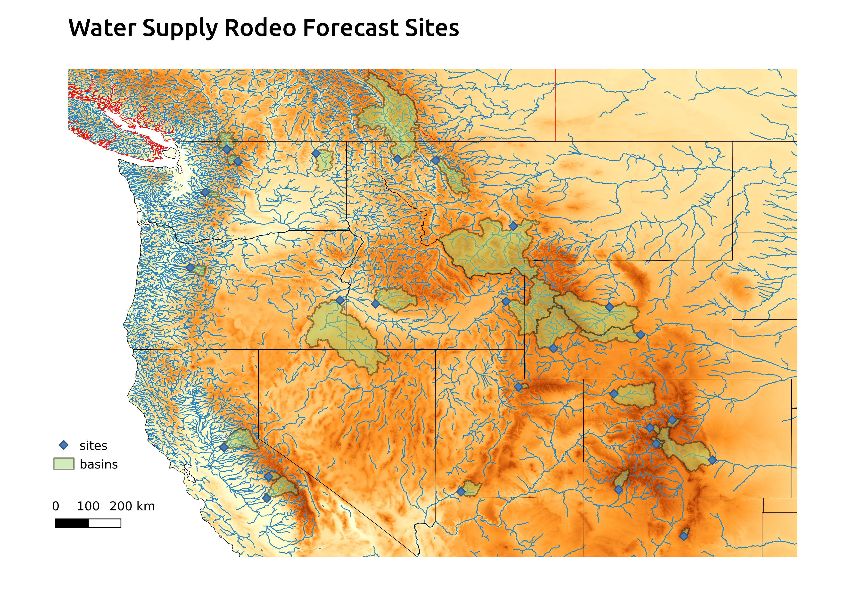

Here is another version using an Albers Equal-Area projection and just showing the map view in QGIS (not a final map layout as above).

Image('./images/WaterSupplyForecastRodeo_Albers.png')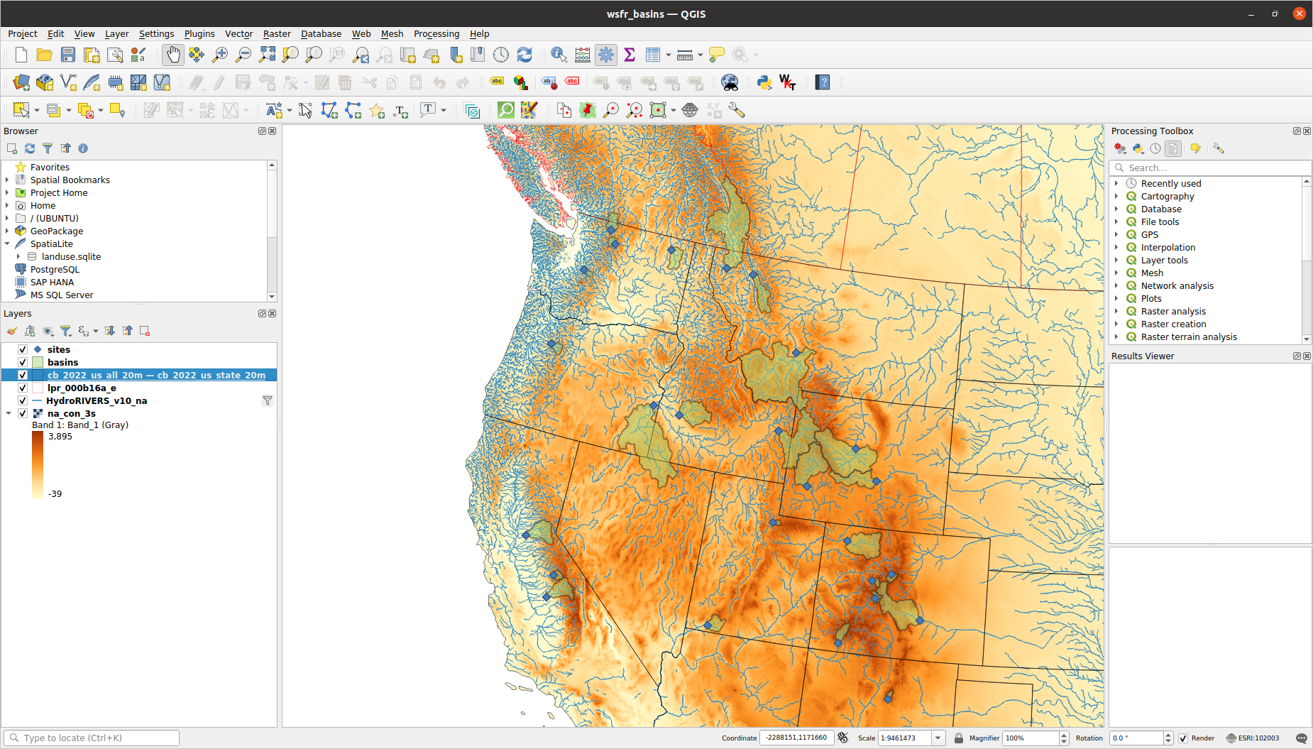

Data sources and Python libraries

(The following is repeated, for convenience, from Part 1)

All of the data we need is freely available. We will need several Python packages for working with the raster and vector data for these maps. In particular, we will use the GeoPandas package to read vector data into GeoDataFrame objects. GeoPandas adds geospatial functionality to pandas.

GeoPandas is an open source project to make working with geospatial data in python easier. GeoPandas extends the datatypes used by pandas to allow spatial operations on geometric types. Geometric operations are performed by shapely. GeoPandas further depends on fiona for file access and matplotlib for plotting.

For raster data, we’ll use the xarray and rioxarray packages.

The xarray package builds on top of NumPy N-d arrays and adds the ability to create and work with labels for the dimensions.

The two main data structures are DataArray (a N-d generalization of a pandas.Series) and DataSet (an N-d generalization of a pandas.DataFrame). The Overview: Why xarray? page has a nice level of detail on the case for xarray and its link to geospatial analysis.

The rioxarray package extends the xarray package to facilitate reading raster data into xarray objects. The actual reading of the raster file is done using another Python package known as rasterio. From the rasterio docs:

Geographic information systems use GeoTIFF and other formats to organize and store gridded raster datasets such as satellite imagery and terrain models. Rasterio reads and writes these formats and provides a Python API based on Numpy N-dimensional arrays and GeoJSON.

Sites and basins (vector)

The streamflow guage sites and associated watershed basins are defined in the geospatial.gpkg GeoPackage file available from the WSFR data downloads page. GeoPackage files can contain multiple layers of both vector and raster data. Individual layers can be read using GeoPandas’ read_file method by passing the layer name. The layer= argument is actually passed along to Fiona, a Python wrapper for accessing vector data via the GDAL/OGR library.

Under the hood, a GeoPackage is a SQLite database that conforms to the GeoPackage standard developed by the Open Geospatial Consortium. Both basins and sites are tables in the GeoPackage (SQLite database) and can be accessed directly with a SQLite database browser or any tool for working with SQLite databases. If you omit the layer= argument, GeoPandas returns the basins layer, likely as it’s the first layer in whatever internal indexing scheme is used with the collection of layers.

import geopandas as gpd

# Reading GeoPackage files
geospatial_input_file = Path(WSFR_DATA_ROOT, 'geospatial.gpkg')
basins_gdf = gpd.read_file(geospatial_input_file, layer='basins')
sites_gdf = gpd.read_file(geospatial_input_file, layer='sites')

basins_gdf

	site_id	name	area	geometry
0	hungry_horse_reservoir_inflow	Hungry Horse Reservoir Inflow	1681.780	POLYGON ((-113.09701 47.24399, -113.09730 47.2...
1	snake_r_nr_heise	Snake River near Heise	5719.410	MULTIPOLYGON (((-110.79196 44.40127, -110.7922...
2	pueblo_reservoir_inflow	Pueblo Reservoir Inflow	4615.460	POLYGON ((-105.67340 38.15883, -105.67315 38.1...
3	sweetwater_r_nr_alcova	Sweetwater River near Alcova	2377.280	POLYGON ((-107.32822 42.21621, -107.32903 42.2...
4	missouri_r_at_toston	Missouri River at Toston	14676.200	POLYGON ((-110.63001 46.30856, -110.63006 46.3...
5	animas_r_at_durango	Animas River at Durango	700.901	POLYGON ((-107.87584 37.27614, -107.87759 37.2...
6	yampa_r_nr_maybell	Yampa River near Maybell	3381.680	MULTIPOLYGON (((-107.02802 40.02615, -107.0277...
7	libby_reservoir_inflow	Libby Reservoir Inflow	9030.450	MULTIPOLYGON (((-114.85817 48.50961, -114.8582...
8	boise_r_nr_boise	Boise River near Boise	2687.340	MULTIPOLYGON (((-115.23528 44.09596, -115.2355...
9	green_r_bl_howard_a_hanson_dam	Green River below Howard Hanson Dam	221.234	POLYGON ((-121.31474 47.13373, -121.31530 47.1...
10	taylor_park_reservoir_inflow	Taylor Park Reservoir Inflow	254.415	MULTIPOLYGON (((-106.74944 39.04268, -106.7499...
11	dillon_reservoir_inflow	Dillon Reservoir Inflow	328.429	POLYGON ((-106.04383 39.35748, -106.04564 39.3...
12	ruedi_reservoir_inflow	Ruedi Reservoir Inflow	223.740	POLYGON ((-106.52087 39.15795, -106.52216 39.1...
13	fontenelle_reservoir_inflow	Fontenelle Reservoir Inflow	4199.150	POLYGON ((-110.06865 42.02568, -110.06944 42.0...
14	weber_r_nr_oakley	Weber River near Oakley	162.429	POLYGON ((-111.06529 40.67623, -111.06633 40.6...
15	san_joaquin_river_millerton_reservoir	San Joaquin River - Millerton Reservoir	1886.720	MULTIPOLYGON (((-120.44227 39.29433, -120.4423...
16	merced_river_yosemite_at_pohono_bridge	Merced River - Yosemite at Pohono Bridge	321.858	POLYGON ((-119.44368 37.86102, -119.44401 37.8...
17	american_river_folsom_lake	American River - Folsom Reservoir	1677.530	MULTIPOLYGON (((-119.52661 37.04015, -119.5265...
18	colville_r_at_kettle_falls	Colville River at Kettle Falls	1086.250	POLYGON ((-117.88747 48.70666, -117.88776 48.7...
19	stehekin_r_at_stehekin	Stehekin River at Stehekin	319.664	POLYGON ((-120.93255 48.19748, -120.93284 48.1...
20	detroit_lake_inflow	Detroit Lake Inflow	452.383	POLYGON ((-121.85271 44.46766, -121.85379 44.4...
21	virgin_r_at_virtin	Virgin River at Virgin	948.039	MULTIPOLYGON (((-112.73274 37.06034, -112.7327...
22	skagit_ross_reservoir	Ross Reservoir Inflow	800.749	MULTIPOLYGON (((-120.98078 48.74358, -120.9810...
23	boysen_reservoir_inflow	Boysen Reservoir Inflow	7706.580	POLYGON ((-108.50590 42.46772, -108.50643 42.4...
24	pecos_r_nr_pecos	Pecos River near Pecos	171.839	MULTIPOLYGON (((-105.50099 35.90638, -105.5007...
25	owyhee_r_bl_owyhee_dam	Owyhee River below Owyhee Dam	11659.800	POLYGON ((-118.19040 43.09658, -118.19034 43.0...

sites_gdf

	site_id	name	geometry
0	hungry_horse_reservoir_inflow	Hungry Horse Reservoir Inflow	POINT (-114.03786 48.35658)
1	snake_r_nr_heise	Snake River near Heise	POINT (-111.66000 43.61250)
2	pueblo_reservoir_inflow	Pueblo Reservoir Inflow	POINT (-104.71803 38.27167)
3	sweetwater_r_nr_alcova	Sweetwater River near Alcova	POINT (-107.13394 42.48996)
4	missouri_r_at_toston	Missouri River at Toston	POINT (-111.42028 46.14657)
5	animas_r_at_durango	Animas River at Durango	POINT (-107.88035 37.27917)
6	yampa_r_nr_maybell	Yampa River near Maybell	POINT (-108.03341 40.50275)
7	libby_reservoir_inflow	Libby Reservoir Inflow	POINT (-115.31872 48.40066)
8	boise_r_nr_boise	Boise River near Boise	POINT (-116.05955 43.52767)
9	green_r_bl_howard_a_hanson_dam	Green River below Howard Hanson Dam	POINT (-121.79789 47.28371)
10	taylor_park_reservoir_inflow	Taylor Park Reservoir Inflow	POINT (-106.60920 38.81833)
11	dillon_reservoir_inflow	Dillon Reservoir Inflow	POINT (-106.06641 39.62554)
12	ruedi_reservoir_inflow	Ruedi Reservoir Inflow	POINT (-106.81865 39.36387)
13	fontenelle_reservoir_inflow	Fontenelle Reservoir Inflow	POINT (-110.06667 42.02778)
14	weber_r_nr_oakley	Weber River near Oakley	POINT (-111.24796 40.73717)
15	san_joaquin_river_millerton_reservoir	San Joaquin River - Millerton Reservoir	POINT (-119.72431 36.98439)
16	merced_river_yosemite_at_pohono_bridge	Merced River - Yosemite at Pohono Bridge	POINT (-119.66567 37.71628)
17	american_river_folsom_lake	American River - Folsom Reservoir	POINT (-121.16436 38.70453)
18	colville_r_at_kettle_falls	Colville River at Kettle Falls	POINT (-118.06249 48.59435)
19	stehekin_r_at_stehekin	Stehekin River at Stehekin	POINT (-120.69177 48.32958)
20	detroit_lake_inflow	Detroit Lake Inflow	POINT (-122.29744 44.75378)
21	virgin_r_at_virtin	Virgin River at Virgin	POINT (-113.18078 37.20415)
22	skagit_ross_reservoir	Ross Reservoir Inflow	POINT (-121.06761 48.73217)
23	boysen_reservoir_inflow	Boysen Reservoir Inflow	POINT (-108.17899 43.42496)
24	pecos_r_nr_pecos	Pecos River near Pecos	POINT (-105.68270 35.70835)
25	owyhee_r_bl_owyhee_dam	Owyhee River below Owyhee Dam	POINT (-117.25583 43.65444)

The total_bounds property gives us a bounding box containing all of the features in that GeoDataFrame. Notice that these are in longitude and latitude and are minx (longitude), miny (latitude), maxx, maxy.

basins_gdf.total_bounds

array([-122.32886555,   35.69784548, -104.7031235 ,   51.33441978])

State and provincial boundaries (vector)

The US government provides Cartographic Boundary Files in both geodatabase and shapefile formats. They are available at different levels of resolution and also by geographic region.

The cartographic boundary files are simplified representations of selected geographic areas from the Census Bureau’s Master Address File/Topologically Integrated Geographic Encoding and Referencing (MAF/TIGER) System. These boundary files are specifically designed for small scale thematic mapping. As of 2019, cartographic boundary files are available in shapefile, geodatabase, and Keyhole Markup Language (KML) format. For more details about these files, including their appropriate usage, please see our Cartographic Boundary File Description page.

I downloaded the lowest resolution (1:20,000,000) zipped geodatabase file of the entire US. Uncompressing it results in a folder that is the geodatabase.

Since some of the basins are in Canada, I found similar maps for Canada in shapefile format.

Later we’ll also use the public domain Natural Earth data.

state_file = Path(WSFR_DATA_ROOT, 'boundaries/cb_2022_us_all_20m.gdb')
state_layer_name = 'cb_2022_us_state_20m'
state_gdf = gpd.read_file(state_file, layer=state_layer_name)

province_file = Path(WSFR_DATA_ROOT, 'boundaries/lpr_000b16a_e/lpr_000b16a_e.shp')
province_gdf = gpd.read_file(province_file)

River layer (vector)

For this layer we can use HydroRIVERS data, a part of the HydroSHEDS project. Both geodatabase and shapefile formats are downloadable from https://www.hydrosheds.org/products/hydrorivers. There are different files for different regions of the world. The North American and Central America data as a zipped geodatabase is available from here and is ~72Mb in size (compressed). Unzip it after downloading. It’s a lot of rivers.

By default, GeoPandas uses fiona as the engine for file reading via the read_file function. According to their docs, they will switch to pyogrio as the default in GeoPandas 1.0 and recommend installing and switching now by using engine='pyogrio'.

conda install -c conda-forge pyogrio

rivers_file = '../data/hydrosheds/HydroRIVERS_v10_na.gdb/HydroRIVERS_v10_na.gdb'
rivers_gdf = gpd.read_file(rivers_file, engine='pyogrio')
rivers_gdf.info()

<class 'geopandas.geodataframe.GeoDataFrame'>
RangeIndex: 986463 entries, 0 to 986462
Data columns (total 16 columns):
 #   Column        Non-Null Count   Dtype   
---  ------        --------------   -----   
 0   HYRIV_ID      986463 non-null  int32   
 1   NEXT_DOWN     986463 non-null  int32   
 2   MAIN_RIV      986463 non-null  int32   
 3   LENGTH_KM     986463 non-null  float32 
 4   DIST_DN_KM    986463 non-null  float32 
 5   DIST_UP_KM    986463 non-null  float32 
 6   CATCH_SKM     986463 non-null  float32 
 7   UPLAND_SKM    986463 non-null  float32 
 8   ENDORHEIC     986463 non-null  int16   
 9   DIS_AV_CMS    986463 non-null  float32 
 10  ORD_STRA      986463 non-null  int16   
 11  ORD_CLAS      986463 non-null  int16   
 12  ORD_FLOW      986463 non-null  int16   
 13  HYBAS_L12     986463 non-null  float64 
 14  Shape_Length  986463 non-null  float64 
 15  geometry      986463 non-null  geometry
dtypes: float32(6), float64(2), geometry(1), int16(4), int32(3)
memory usage: 64.0 MB

Let’s filter by ORD_FLOW to reduce the number of features to plot.

rivers_gdf = rivers_gdf.query('ORD_FLOW <= 6')
rivers_gdf.info()

<class 'geopandas.geodataframe.GeoDataFrame'>
Index: 299372 entries, 6 to 986458
Data columns (total 16 columns):
 #   Column        Non-Null Count   Dtype   
---  ------        --------------   -----   
 0   HYRIV_ID      299372 non-null  int32   
 1   NEXT_DOWN     299372 non-null  int32   
 2   MAIN_RIV      299372 non-null  int32   
 3   LENGTH_KM     299372 non-null  float32 
 4   DIST_DN_KM    299372 non-null  float32 
 5   DIST_UP_KM    299372 non-null  float32 
 6   CATCH_SKM     299372 non-null  float32 
 7   UPLAND_SKM    299372 non-null  float32 
 8   ENDORHEIC     299372 non-null  int16   
 9   DIS_AV_CMS    299372 non-null  float32 
 10  ORD_STRA      299372 non-null  int16   
 11  ORD_CLAS      299372 non-null  int16   
 12  ORD_FLOW      299372 non-null  int16   
 13  HYBAS_L12     299372 non-null  float64 
 14  Shape_Length  299372 non-null  float64 
 15  geometry      299372 non-null  geometry
dtypes: float32(6), float64(2), geometry(1), int16(4), int32(3)
memory usage: 21.7 MB

DEM layer (raster)

Since this project is all about hydrology, we will use a “hydrologically conditioned DEM” available as part of the HydroSHEDS core layer.

• go to https://www.hydrosheds.org/hydrosheds-core-downloads,
• select the Conditioned DEM tab near bottom of page,
• download the compressed file for North and Central America; it’s ~2.7GB,
• uncompress the downloaded file and you’ll get a folder containing documentation and the GeoTIFF file, na_con_3s.tif, with the DEM raster.

Since this is raster data in a GeoTIFF file, we can use the rioxarray package to read this data into an xarray DataArray.

import rioxarray

dem_file = Path(WSFR_DATA_ROOT, 'hydrosheds/na_con_3s/na_con_3s.tif')
dem_xr = rioxarray.open_rasterio(dem_file, masked=True)
dem_xr

<xarray.DataArray (band: 1, y: 72000, x: 120000)>
[8640000000 values with dtype=float32]
Coordinates:
  * band         (band) int64 1
  * x            (x) float64 -150.0 -150.0 -150.0 -150.0 ... -50.0 -50.0 -50.0
  * y            (y) float64 60.0 60.0 60.0 60.0 ... 0.002083 0.00125 0.0004167
    spatial_ref  int64 0
Attributes:
    AREA_OR_POINT:       Area
    RepresentationType:  THEMATIC
    scale_factor:        1.0
    add_offset:          0.0
    long_name:           Band_1

xarray.DataArray

• band: 1
• y: 72000
• x: 120000

• ...

  [8640000000 values with dtype=float32]

• Coordinates: (4)
  • band
    (band)
    int64
    1

    array([1])

  • x
    (x)
    float64
    -150.0 -150.0 ... -50.0 -50.0

    array([-149.999583, -149.99875 , -149.997917, ...,  -50.002083,  -50.00125 ,
            -50.000417])

  • y
    (y)
    float64
    60.0 60.0 ... 0.00125 0.0004167

    array([5.999958e+01, 5.999875e+01, 5.999792e+01, ..., 2.083333e-03,
           1.250000e-03, 4.166667e-04])

  • spatial_ref
    ()
    int64
    0

    crs_wkt :

    GEOGCS["WGS 84",DATUM["WGS_1984",SPHEROID["WGS 84",6378137,298.257223563,AUTHORITY["EPSG","7030"]],AUTHORITY["EPSG","6326"]],PRIMEM["Greenwich",0,AUTHORITY["EPSG","8901"]],UNIT["degree",0.0174532925199433,AUTHORITY["EPSG","9122"]],AXIS["Latitude",NORTH],AXIS["Longitude",EAST],AUTHORITY["EPSG","4326"]]

    semi_major_axis :

    6378137.0

    semi_minor_axis :

    6356752.314245179

    inverse_flattening :

    298.257223563

    reference_ellipsoid_name :

    WGS 84

    longitude_of_prime_meridian :

    0.0

    prime_meridian_name :

    Greenwich

    geographic_crs_name :

    WGS 84

    horizontal_datum_name :

    World Geodetic System 1984

    grid_mapping_name :

    latitude_longitude

    spatial_ref :

    GEOGCS["WGS 84",DATUM["WGS_1984",SPHEROID["WGS 84",6378137,298.257223563,AUTHORITY["EPSG","7030"]],AUTHORITY["EPSG","6326"]],PRIMEM["Greenwich",0,AUTHORITY["EPSG","8901"]],UNIT["degree",0.0174532925199433,AUTHORITY["EPSG","9122"]],AXIS["Latitude",NORTH],AXIS["Longitude",EAST],AUTHORITY["EPSG","4326"]]

    GeoTransform :

    -150.0 0.000833333333333333 0.0 59.99999999999999 0.0 -0.000833333333333333

    array(0)

• Indexes: (3)
  • band
    PandasIndex

    PandasIndex(Index([1], dtype='int64', name='band'))

  • x
    PandasIndex

    PandasIndex(Index([-149.99958333333333,          -149.99875, -149.99791666666667,
           -149.99708333333334,          -149.99625, -149.99541666666667,
           -149.99458333333334,          -149.99375, -149.99291666666667,
           -149.99208333333334,
           ...
           -50.007916666666716, -50.007083333333384,  -50.00625000000005,
            -50.00541666666672, -50.004583333333386,  -50.00375000000004,
            -50.00291666666671, -50.002083333333374,  -50.00125000000004,
            -50.00041666666671],
          dtype='float64', name='x', length=120000))

  • y
    PandasIndex

    PandasIndex(Index([    59.99958333333333,    59.998749999999994,     59.99791666666666,
               59.99708333333333,    59.996249999999996,     59.99541666666666,
              59.994583333333324,     59.99374999999999,     59.99291666666666,
              59.992083333333326,
           ...
            0.007916666666687888,  0.007083333333355313,  0.006250000000022737,
            0.005416666666690162,  0.004583333333350481, 0.0037500000000179057,
           0.0029166666666853303,  0.002083333333352755, 0.0012500000000201794,
            0.000416666666687604],
          dtype='float64', name='y', length=72000))

• Attributes: (5)

  AREA_OR_POINT :

  Area

  RepresentationType :

  THEMATIC

  scale_factor :

  1.0

  add_offset :

  0.0

  long_name :

  Band_1

print(f'Number of cells: {dem_xr.shape[1] * dem_xr.shape[2]:,}')

Number of cells: 8,640,000,000

Yikes! That is one big array. This is a DEM for all of North and Central America and we only need a portion. I used QGIS to get an approximate extent for the map we want to make. Then we can use rioxarray to clip the raster.

# Extent is minx, miny, maxx, maxy
extent_epsg_4326 = [-126, 35, -103, 52] 
minx_4326, miny_4326, maxx_4326, maxy_4326 = extent_epsg_4326

dem_xr = dem_xr.rio.clip_box(
            minx=minx_4326,
            miny=miny_4326,
            maxx=maxx_4326,
            maxy=maxy_4326,
            crs="EPSG:4326",
        )

print(f'bounds: {dem_xr.rio.bounds()}')
print(f'shape: {dem_xr.shape}')
print(f'number of cells: {dem_xr.shape[1] * dem_xr.shape[2]:,}')

bounds: (-126.00000000000001, 35.0, -102.9991666666667, 52.00083333333333)
shape: (1, 20401, 27601)
number of cells: 563,088,001

That’s still a huge array and I’m thinking this is going to be problematic. I’m far from clear on how different Python based plotting libraries handle large raster files. We’ll deal with this when we get to it. First, we have another issue to deal with.

Preparation for map making

In the previous section we read all of the data into appropriate data structures - the vector layers (sites, basins, rivers, and state/province boundaries) were stored in GeoDataFrame objects and the DEM raster layer was stored in an xarray DataArray.

But, before we can try to plot all of this data together on a map, we need to make sure that all of the data uses the same projected coordinate reference system so that everything shows up where it should on the map. We won’t have QGIS to magically reproject data as needed in order to create a map.

What is the coordinate reference system (CRS) for each of our data items? The GeoDataFrame objects have a crs property that can be checked. For the raster, we can use the rio accessor from rioxarray to access the crs property of the DataArray.

# Vector GeoDataFrames
print(f'sites CRS: {sites_gdf.crs}')
print(f'basins CRS: {basins_gdf.crs}')
print(f'state CRS: {state_gdf.crs}')
print(f'province CRS: {province_gdf.crs}')
print(f'rivers CRS: {rivers_gdf.crs}')

# Raster DataArray
print(f'DEM CRS: {dem_xr.rio.crs}')

sites CRS: EPSG:4326
basins CRS: EPSG:4326
state CRS: EPSG:4269
province CRS: PROJCS["PCS_Lambert_Conformal_Conic",GEOGCS["NAD83",DATUM["North_American_Datum_1983",SPHEROID["GRS 1980",6378137,298.257222101,AUTHORITY["EPSG","7019"]],AUTHORITY["EPSG","6269"]],PRIMEM["Greenwich",0],UNIT["Degree",0.0174532925199433]],PROJECTION["Lambert_Conformal_Conic_2SP"],PARAMETER["latitude_of_origin",63.390675],PARAMETER["central_meridian",-91.8666666666667],PARAMETER["standard_parallel_1",49],PARAMETER["standard_parallel_2",77],PARAMETER["false_easting",6200000],PARAMETER["false_northing",3000000],UNIT["metre",1,AUTHORITY["EPSG","9001"]],AXIS["Easting",EAST],AXIS["Northing",NORTH]]
rivers CRS: EPSG:4326
DEM CRS: EPSG:4326

A few of the data items use the EPSG:4326 CRS, the state data uses EPSG:4269 and the province data uses the Lambert Conformal Conic projection. Now what?

A bit on coordinate reference systems and projections

This booklet written by ESRI is a nice primer on coordinate reference systems and projections. Chapter 2 of the online PyGIS book is another source of introductory information on these topics.

EPSG:4326, a very commonly used CRS, is a geographic coordinate system and not a projected coordinate system.

A good explanation of the difference between these two things is provided by ESRI.

• A GCS defines where the data is located on the earth’s surface.
• A PCS tells the data how to draw on a flat surface, like on a paper map or a computer screen.

and

A projected coordinate system (PCS) is a GCS that has been flattened using a map projection.

The EPSG:4326 CRS uses longitude and latitude to locate points on an underlying model of the earth (WGS84). But, this is a 3D model and any attempt to represent it in 2D (via one of countless possible projections) will lead to different degrees of distortion in area, distance and angle conformance. Before plotting geographic data on some 2D surface (e.g. screen or paper) we need to pick an appropriate projected coordinate reference system. BTW, sometimes it seems like EPSG:4326 and WGS84 are used synonomously. The folks at the MapScaping podcast have done a nice blog post on the relationship between EPSG:4326 and WGS84.

We could simply plot the EPSG:4326 data on an xy-grid with Matplotlib. Implicitly we have used a pseudo Plate Carree or equirectangular projection (“pseudo” because it’s measured in degrees instead of meters). This might be acceptable for very small areas or if you’re just interested in a rough map and don’t need to do distance or area calculations. This “non-projection” is referenced in the PROJ documentation as a projection that leaves the underlying CRS unchanged - it’s just a pass through.

But, didn’t we just create a map in QGIS in which all layers used the EPSG:4326 CRS? When QGIS displays the map on the screen, it must do some sort of projection. How does QGIS handle projections and CRS for individual layers and the map display? According to this docs page each layer can have its own CRS and the overall project has a CRS. The project CRS controls how the map is displayed and QGIS does “on the fly” reprojections of individual layers as needed. The individual layer CRS’s define the locations (XY) in each layer - often EPSG:4326 which is NOT a projected CRS. By default, the project CRS is also EPSG:4326. This GIS StackExchange post as well as this one were also quite helpful in answering this question.

The interplay (both generally and within a GIS) of datums, coordinate reference systems and projections is a complex topic. Here are a few general resources that I have found to be helpful.

• GIS Fundamentals: A First Text on Geographic Information Systems - textbook by Paul Bolstad
• PROJ - THE software tool for transformations between CRS
• Understanding Map Projections - booklet produced by ESRI
• Spatial references, coordinate systems, projections, datums, ellipsoids – confusing? - blog post that tries to cut through the confusion
• Reprojecting geographic features - web page by Bill Huber
• What is a CRS? - a chapter in the online PyGIS book
• Reprojecting and transforming data - part of the QGIS Training Manual in the chapter on vector analysis
• EPSG 3857 or 4326 for Web Mapping - GIS StackExchange question discusses GCS vs PCS for two common EPSG codes
• Projecting EPSG:4326 data in 2D map - GIS StackExchange question that gets into some interesting projection related subtleties and anecdotes.
• Coordinate reference systems: background - very detailed history of PROJ, GDAL and their use in R and other systems.

Which projection to use?

For the continential US, the USGS uses a number of different projections. We will use the Albers Equal-Area Conic projection (AEA) - it’s the one used by the USGS for state and regional maps. The PROJ page for AEA includes the official proj-string.

It’s a bit more complicated as there are multiple versions of AEA developed by the USGS (e.g. CONUS and Alaska have separate versions). Instead of an EPSG code for AEA, there appears to be an ESRI code, ESRI:102008 for the North American AEA. For other versions, there are different EPSG codes:

• CONUS (USGS version) - EPSG:5070
• Alaska - EPSG:3338
• Hawaii - no registered EPSG code

Since our map is focused on the western United States and a bit of Canada, we’ll use ESRI:102008.

What exactly are the differences between EPSG:5070 and the AEA projection ESRI:102008? To answer this question we need to look at the detailed specifications of each projection. We can do this by examining what are known as well known text (WKT) representations of CRSs. How do we get the WKT representations of a giving CRS? Turns out that the crs property in a GeoDataFrame isn’t just a string, but is a pyproj.CRS object and this object knows about WKTs.

The pyproj package is a Python interface to PROJ. One of the things we can do with a pyproj.CRS object is get a WKT representation of it using the to_wkt() method. The WKT representation contains a wealth of detailed data that define a projection. Our goal here is just to see if we can use the WKTs to figure out the difference between the USGS version of AEA and the ESRI:102008 version.

from pyproj import CRS

Here’s the North American Albers Equal Area.

crs_102008 = CRS.from_string("ESRI:102008")
wkt_102008 = crs_102008.to_wkt()
print(crs_102008.to_wkt(pretty=True)) 

PROJCRS["North_America_Albers_Equal_Area_Conic",
    BASEGEOGCRS["NAD83",
        DATUM["North American Datum 1983",
            ELLIPSOID["GRS 1980",6378137,298.257222101,
                LENGTHUNIT["metre",1]]],
        PRIMEM["Greenwich",0,
            ANGLEUNIT["degree",0.0174532925199433]],
        ID["EPSG",4269]],
    CONVERSION["North_America_Albers_Equal_Area_Conic",
        METHOD["Albers Equal Area",
            ID["EPSG",9822]],
        PARAMETER["Latitude of false origin",40,
            ANGLEUNIT["degree",0.0174532925199433],
            ID["EPSG",8821]],
        PARAMETER["Longitude of false origin",-96,
            ANGLEUNIT["degree",0.0174532925199433],
            ID["EPSG",8822]],
        PARAMETER["Latitude of 1st standard parallel",20,
            ANGLEUNIT["degree",0.0174532925199433],
            ID["EPSG",8823]],
        PARAMETER["Latitude of 2nd standard parallel",60,
            ANGLEUNIT["degree",0.0174532925199433],
            ID["EPSG",8824]],
        PARAMETER["Easting at false origin",0,
            LENGTHUNIT["metre",1],
            ID["EPSG",8826]],
        PARAMETER["Northing at false origin",0,
            LENGTHUNIT["metre",1],
            ID["EPSG",8827]]],
    CS[Cartesian,2],
        AXIS["(E)",east,
            ORDER[1],
            LENGTHUNIT["metre",1]],
        AXIS["(N)",north,
            ORDER[2],
            LENGTHUNIT["metre",1]],
    USAGE[
        SCOPE["Not known."],
        AREA["North America - onshore and offshore: Canada - Alberta; British Columbia; Manitoba; New Brunswick; Newfoundland and Labrador; Northwest Territories; Nova Scotia; Nunavut; Ontario; Prince Edward Island; Quebec; Saskatchewan; Yukon. United States (USA) - Alabama; Alaska (mainland); Arizona; Arkansas; California; Colorado; Connecticut; Delaware; Florida; Georgia; Idaho; Illinois; Indiana; Iowa; Kansas; Kentucky; Louisiana; Maine; Maryland; Massachusetts; Michigan; Minnesota; Mississippi; Missouri; Montana; Nebraska; Nevada; New Hampshire; New Jersey; New Mexico; New York; North Carolina; North Dakota; Ohio; Oklahoma; Oregon; Pennsylvania; Rhode Island; South Carolina; South Dakota; Tennessee; Texas; Utah; Vermont; Virginia; Washington; West Virginia; Wisconsin; Wyoming."],
        BBOX[23.81,-172.54,86.46,-47.74]],
    ID["ESRI",102008]]

… and here’s the EPSG:5070 version:

crs_5070 = CRS.from_string('EPSG:5070')
print(crs_5070.to_wkt(pretty=True))

PROJCRS["NAD83 / Conus Albers",
    BASEGEOGCRS["NAD83",
        DATUM["North American Datum 1983",
            ELLIPSOID["GRS 1980",6378137,298.257222101,
                LENGTHUNIT["metre",1]]],
        PRIMEM["Greenwich",0,
            ANGLEUNIT["degree",0.0174532925199433]],
        ID["EPSG",4269]],
    CONVERSION["Conus Albers",
        METHOD["Albers Equal Area",
            ID["EPSG",9822]],
        PARAMETER["Latitude of false origin",23,
            ANGLEUNIT["degree",0.0174532925199433],
            ID["EPSG",8821]],
        PARAMETER["Longitude of false origin",-96,
            ANGLEUNIT["degree",0.0174532925199433],
            ID["EPSG",8822]],
        PARAMETER["Latitude of 1st standard parallel",29.5,
            ANGLEUNIT["degree",0.0174532925199433],
            ID["EPSG",8823]],
        PARAMETER["Latitude of 2nd standard parallel",45.5,
            ANGLEUNIT["degree",0.0174532925199433],
            ID["EPSG",8824]],
        PARAMETER["Easting at false origin",0,
            LENGTHUNIT["metre",1],
            ID["EPSG",8826]],
        PARAMETER["Northing at false origin",0,
            LENGTHUNIT["metre",1],
            ID["EPSG",8827]]],
    CS[Cartesian,2],
        AXIS["easting (X)",east,
            ORDER[1],
            LENGTHUNIT["metre",1]],
        AXIS["northing (Y)",north,
            ORDER[2],
            LENGTHUNIT["metre",1]],
    USAGE[
        SCOPE["Data analysis and small scale data presentation for contiguous lower 48 states."],
        AREA["United States (USA) - CONUS onshore - Alabama; Arizona; Arkansas; California; Colorado; Connecticut; Delaware; Florida; Georgia; Idaho; Illinois; Indiana; Iowa; Kansas; Kentucky; Louisiana; Maine; Maryland; Massachusetts; Michigan; Minnesota; Mississippi; Missouri; Montana; Nebraska; Nevada; New Hampshire; New Jersey; New Mexico; New York; North Carolina; North Dakota; Ohio; Oklahoma; Oregon; Pennsylvania; Rhode Island; South Carolina; South Dakota; Tennessee; Texas; Utah; Vermont; Virginia; Washington; West Virginia; Wisconsin; Wyoming."],
        BBOX[24.41,-124.79,49.38,-66.91]],
    ID["EPSG",5070]]

To highlight the differences between these two strings, we can use Python’s difflib package. It’s kind of like the Linux diff command but in Python.

from difflib import ndiff

diff = ndiff(crs_102008.to_wkt(pretty=True).splitlines(), crs_5070.to_wkt(pretty=True).splitlines())
for line in diff:
    print(line)

- PROJCRS["North_America_Albers_Equal_Area_Conic",
+ PROJCRS["NAD83 / Conus Albers",
      BASEGEOGCRS["NAD83",
          DATUM["North American Datum 1983",
              ELLIPSOID["GRS 1980",6378137,298.257222101,
                  LENGTHUNIT["metre",1]]],
          PRIMEM["Greenwich",0,
              ANGLEUNIT["degree",0.0174532925199433]],
          ID["EPSG",4269]],
-     CONVERSION["North_America_Albers_Equal_Area_Conic",
+     CONVERSION["Conus Albers",
          METHOD["Albers Equal Area",
              ID["EPSG",9822]],
-         PARAMETER["Latitude of false origin",40,
?                                              ^^

+         PARAMETER["Latitude of false origin",23,
?                                              ^^

              ANGLEUNIT["degree",0.0174532925199433],
              ID["EPSG",8821]],
          PARAMETER["Longitude of false origin",-96,
              ANGLEUNIT["degree",0.0174532925199433],
              ID["EPSG",8822]],
-         PARAMETER["Latitude of 1st standard parallel",20,
?                                                        ^

+         PARAMETER["Latitude of 1st standard parallel",29.5,
?                                                        ^^^

              ANGLEUNIT["degree",0.0174532925199433],
              ID["EPSG",8823]],
-         PARAMETER["Latitude of 2nd standard parallel",60,
?                                                       ^^

+         PARAMETER["Latitude of 2nd standard parallel",45.5,
?                                                       ^^^^

              ANGLEUNIT["degree",0.0174532925199433],
              ID["EPSG",8824]],
          PARAMETER["Easting at false origin",0,
              LENGTHUNIT["metre",1],
              ID["EPSG",8826]],
          PARAMETER["Northing at false origin",0,
              LENGTHUNIT["metre",1],
              ID["EPSG",8827]]],
      CS[Cartesian,2],
-         AXIS["(E)",east,
?                ^

+         AXIS["easting (X)",east,
?               ++++++++ ^

              ORDER[1],
              LENGTHUNIT["metre",1]],
-         AXIS["(N)",north,
?                ^

+         AXIS["northing (Y)",north,
?               +++++++++ ^

              ORDER[2],
              LENGTHUNIT["metre",1]],
      USAGE[
-         SCOPE["Not known."],
+         SCOPE["Data analysis and small scale data presentation for contiguous lower 48 states."],
-         AREA["North America - onshore and offshore: Canada - Alberta; British Columbia; Manitoba; New Brunswick; Newfoundland and Labrador; Northwest Territories; Nova Scotia; Nunavut; Ontario; Prince Edward Island; Quebec; Saskatchewan; Yukon. United States (USA) - Alabama; Alaska (mainland); Arizona; Arkansas; California; Colorado; Connecticut; Delaware; Florida; Georgia; Idaho; Illinois; Indiana; Iowa; Kansas; Kentucky; Louisiana; Maine; Maryland; Massachusetts; Michigan; Minnesota; Mississippi; Missouri; Montana; Nebraska; Nevada; New Hampshire; New Jersey; New Mexico; New York; North Carolina; North Dakota; Ohio; Oklahoma; Oregon; Pennsylvania; Rhode Island; South Carolina; South Dakota; Tennessee; Texas; Utah; Vermont; Virginia; Washington; West Virginia; Wisconsin; Wyoming."],
?               ^^^^^^^^^^^^^^^^^^^^^^^^^^^^^^^^^^^^^^^^^^^^^^^^^^^^^^^^^^^^^^^^^^^^^^^^^^^^^^^^^^^^^^^^^^^^^^^^^^^^^^^^^^^^^^^^^^^^^^^^^^^^^^^^^^^^^^^^^^^^^^^^^^^^^^^^^  ^^^^^^^^^^^^^^^^^^^^^^^^^^^^^^^^^^^^^^^^^^^^^^^^^^^^^^^^^^^^^^^^^^^^^^^^^^^^^^^^^^^^^^^^^                   ^^^^^^^^^^^^^^^^^   ^^^^^^^^^^^^^^^^

+         AREA["United States (USA) - CONUS onshore - Alabama; Arizona; Arkansas; California; Colorado; Connecticut; Delaware; Florida; Georgia; Idaho; Illinois; Indiana; Iowa; Kansas; Kentucky; Louisiana; Maine; Maryland; Massachusetts; Michigan; Minnesota; Mississippi; Missouri; Montana; Nebraska; Nevada; New Hampshire; New Jersey; New Mexico; New York; North Carolina; North Dakota; Ohio; Oklahoma; Oregon; Pennsylvania; Rhode Island; South Carolina; South Dakota; Tennessee; Texas; Utah; Vermont; Virginia; Washington; West Virginia; Wisconsin; Wyoming."],
?               ^^^^^^  ^^^^^         ++++++++++++++++          ^^^^^^^   ^^^^^^^

-         BBOX[23.81,-172.54,86.46,-47.74]],
+         BBOX[24.41,-124.79,49.38,-66.91]],
-     ID["ESRI",102008]]
?           ^^  ^ ^ --

+     ID["EPSG",5070]]
?          + ^  ^ ^

So, the significant differences are:

• different origins of latitude and longitude
• different standard parallels
• different areas of applicability (see SCOPE and BBOX)

Notice that the WKT for EPSG:4326 contains no conversion related parameters as it is NOT a projected coordinated reference system.

print(sites_gdf.crs.to_wkt(pretty=True))

GEOGCRS["WGS 84",
    ENSEMBLE["World Geodetic System 1984 ensemble",
        MEMBER["World Geodetic System 1984 (Transit)"],
        MEMBER["World Geodetic System 1984 (G730)"],
        MEMBER["World Geodetic System 1984 (G873)"],
        MEMBER["World Geodetic System 1984 (G1150)"],
        MEMBER["World Geodetic System 1984 (G1674)"],
        MEMBER["World Geodetic System 1984 (G1762)"],
        MEMBER["World Geodetic System 1984 (G2139)"],
        ELLIPSOID["WGS 84",6378137,298.257223563,
            LENGTHUNIT["metre",1]],
        ENSEMBLEACCURACY[2.0]],
    PRIMEM["Greenwich",0,
        ANGLEUNIT["degree",0.0174532925199433]],
    CS[ellipsoidal,2],
        AXIS["geodetic latitude (Lat)",north,
            ORDER[1],
            ANGLEUNIT["degree",0.0174532925199433]],
        AXIS["geodetic longitude (Lon)",east,
            ORDER[2],
            ANGLEUNIT["degree",0.0174532925199433]],
    USAGE[
        SCOPE["Horizontal component of 3D system."],
        AREA["World."],
        BBOX[-90,-180,90,180]],
    ID["EPSG",4326]]

Ok, we are going to use ESRI:102008 as our common projected CRS for all of our data items.

Some additional resources on choosing projections include:

• Choose the right projection (ESRI)
• Which projection for CONUS? (GIS StackExchange)
• epsg:3857 or epsg:4326 for web mapping? (GIS StackExchange)

Reprojecting to ESRI:102008

Let’s try to change the CRS for all of our data items to the Albers Equal-Area (USGS) CRS. For the GeoDataFrame objects, the to_crs method accepts EPSG codes.

sites_102008_gdf = sites_gdf.to_crs(crs_102008)
print(f'sites CRS: {sites_102008_gdf.crs}')
basins_102008_gdf = basins_gdf.to_crs(crs_102008)
print(f'basins CRS: {basins_102008_gdf.crs}')
state_102008_gdf = state_gdf.to_crs(crs_102008)
print(f'state CRS: {state_102008_gdf.crs}')
province_102008_gdf = province_gdf.to_crs(crs_102008)
print(f'province CRS: {province_102008_gdf.crs}')
rivers_102008_gdf = rivers_gdf.to_crs(crs_102008)
print(f'rivers CRS: {rivers_102008_gdf.crs}')

sites CRS: ESRI:102008
basins CRS: ESRI:102008
state CRS: ESRI:102008
province CRS: ESRI:102008
rivers CRS: ESRI:102008

Now we need to do the same for the DEM.

To do this, looks like we need rio.reproject. Reprojecting rasters can be computationally intensive, but we need to do it if we want our data to align properly on our map. We clipped the DEM raster earlier and this will make the reprojection easier. A few helpful links on doing reprojection with rioxarray include:

• Reprojection section in rasterio docs
• API for rio.reproject
• Reprojecting a large raster using Python and rasterio

The rio.reproject() function allows you to both resample and reproject a raster with a single function call. It’s just a wrapper for rasterio.wrap.reproject.

I followed the lead of this blog post - Upsample and Downsample raster in python using rioxarray.

import rasterio

downscale_factor = 1/10
 
# Calculate new height and width using downscale_factor
new_width = dem_xr.rio.width * downscale_factor
new_height = dem_xr.rio.height * downscale_factor
print(int(new_width), int(new_height))

2760 2040

We can resample and reproject from EPSG:4326 to ESRI:102008. I would assume that the resampling would take place first followed by the projection.

I’m also not sure about what makes the most sense for the no data value. Our original data is all integer and the no data value is 32767 (EPSG:4326). For ESRI:102008, the no data value is -9999. However, after resampling, the array values could be floats depending on how the resampling is done.

The rasterio.warp.reproject() function will determine the src_nodata value from the dem_xr rioaxarray and these pixel values won’t get used during resampling.

A few helpful resources on no data values in raster files are:

• Nodata management from rioxarray docs
• Downsides to saving rasters with nan as no data values

Now we are ready to resample and reproject by passing in our target projection, a resampling scheme, and the new shape of our target raster.

# Resample and reproject
dem_102008_xr = dem_xr.rio.reproject('ESRI:102008', resampling=rasterio.enums.Resampling.bilinear,
                                     shape=(int(new_height), int(new_width))) 
dem_102008_xr

<xarray.DataArray (band: 1, y: 2040, x: 2760)>
array([[[nan, nan, nan, ..., nan, nan, nan],
        [nan, nan, nan, ..., nan, nan, nan],
        [nan, nan, nan, ..., nan, nan, nan],
        ...,
        [nan, nan, nan, ..., nan, nan, nan],
        [nan, nan, nan, ..., nan, nan, nan],
        [nan, nan, nan, ..., nan, nan, nan]]], dtype=float32)
Coordinates:
  * x            (x) float64 -2.554e+06 -2.553e+06 ... -4.589e+05 -4.581e+05
  * y            (y) float64 1.722e+06 1.721e+06 ... -5.636e+05 -5.647e+05
  * band         (band) int64 1
    spatial_ref  int64 0
Attributes:
    AREA_OR_POINT:       Area
    RepresentationType:  THEMATIC
    scale_factor:        1.0
    add_offset:          0.0
    long_name:           Band_1

xarray.DataArray

• band: 1
• y: 2040
• x: 2760

• nan nan nan nan nan nan nan nan ... nan nan nan nan nan nan nan nan

  array([[[nan, nan, nan, ..., nan, nan, nan],
          [nan, nan, nan, ..., nan, nan, nan],
          [nan, nan, nan, ..., nan, nan, nan],
          ...,
          [nan, nan, nan, ..., nan, nan, nan],
          [nan, nan, nan, ..., nan, nan, nan],
          [nan, nan, nan, ..., nan, nan, nan]]], dtype=float32)

• Coordinates: (4)
  • x
    (x)
    float64
    -2.554e+06 ... -4.581e+05

    axis :

    X

    long_name :

    x coordinate of projection

    standard_name :

    projection_x_coordinate

    units :

    metre

    array([-2553828.668114, -2553069.081085, -2552309.494056, ...,  -459647.229615,
            -458887.642587,  -458128.055558])

  • y
    (y)
    float64
    1.722e+06 1.721e+06 ... -5.647e+05

    axis :

    Y

    long_name :

    y coordinate of projection

    standard_name :

    projection_y_coordinate

    units :

    metre

    array([1721937.725242, 1720816.28022 , 1719694.835198, ..., -562445.783991,
           -563567.229013, -564688.674035])

  • band
    (band)
    int64
    1

    array([1])

  • spatial_ref
    ()
    int64
    0

    crs_wkt :

    PROJCS["North_America_Albers_Equal_Area_Conic",GEOGCS["NAD83",DATUM["North_American_Datum_1983",SPHEROID["GRS 1980",6378137,298.257222101,AUTHORITY["EPSG","7019"]],AUTHORITY["EPSG","6269"]],PRIMEM["Greenwich",0,AUTHORITY["EPSG","8901"]],UNIT["degree",0.0174532925199433,AUTHORITY["EPSG","9122"]],AUTHORITY["EPSG","4269"]],PROJECTION["Albers_Conic_Equal_Area"],PARAMETER["latitude_of_center",40],PARAMETER["longitude_of_center",-96],PARAMETER["standard_parallel_1",20],PARAMETER["standard_parallel_2",60],PARAMETER["false_easting",0],PARAMETER["false_northing",0],UNIT["metre",1,AUTHORITY["EPSG","9001"]],AXIS["Easting",EAST],AXIS["Northing",NORTH],AUTHORITY["ESRI","102008"]]

    semi_major_axis :

    6378137.0

    semi_minor_axis :

    6356752.314140356

    inverse_flattening :

    298.257222101

    reference_ellipsoid_name :

    GRS 1980

    longitude_of_prime_meridian :

    0.0

    prime_meridian_name :

    Greenwich

    geographic_crs_name :

    NAD83

    horizontal_datum_name :

    North American Datum 1983

    projected_crs_name :

    North_America_Albers_Equal_Area_Conic

    grid_mapping_name :

    albers_conical_equal_area

    standard_parallel :

    (20.0, 60.0)

    latitude_of_projection_origin :

    40.0

    longitude_of_central_meridian :

    -96.0

    false_easting :

    0.0

    false_northing :

    0.0

    spatial_ref :

    PROJCS["North_America_Albers_Equal_Area_Conic",GEOGCS["NAD83",DATUM["North_American_Datum_1983",SPHEROID["GRS 1980",6378137,298.257222101,AUTHORITY["EPSG","7019"]],AUTHORITY["EPSG","6269"]],PRIMEM["Greenwich",0,AUTHORITY["EPSG","8901"]],UNIT["degree",0.0174532925199433,AUTHORITY["EPSG","9122"]],AUTHORITY["EPSG","4269"]],PROJECTION["Albers_Conic_Equal_Area"],PARAMETER["latitude_of_center",40],PARAMETER["longitude_of_center",-96],PARAMETER["standard_parallel_1",20],PARAMETER["standard_parallel_2",60],PARAMETER["false_easting",0],PARAMETER["false_northing",0],UNIT["metre",1,AUTHORITY["EPSG","9001"]],AXIS["Easting",EAST],AXIS["Northing",NORTH],AUTHORITY["ESRI","102008"]]

    GeoTransform :

    -2554208.4616283686 759.5870288351857 0.0 1722498.447752379 0.0 -1121.4450217146702

    array(0)

• Indexes: (3)
  • x
    PandasIndex

    PandasIndex(Index([ -2553828.668113951,  -2553069.081085116, -2552309.4940562807,
           -2551549.9070274457, -2550790.3199986103, -2550030.7329697753,
             -2549271.14594094,  -2548511.558912105, -2547751.9718832695,
           -2546992.3848544345,
           ...
            -464964.3388171904,  -464204.7517883552,    -463445.16475952,
            -462685.5777306848,  -461925.9907018496, -461166.40367301437,
           -460406.81664417917, -459647.22961534397,   -458887.642586509,
            -458128.0555576738],
          dtype='float64', name='x', length=2760))

  • y
    PandasIndex

    PandasIndex(Index([1721937.7252415218,  1720816.280219807, 1719694.8351980925,
           1718573.3901763777, 1717451.9451546632, 1716330.5001329484,
           1715209.0551112338,  1714087.610089519, 1712966.1650678045,
           1711844.7200460897,
           ...
           -554595.6688392586, -555717.1138609736, -556838.5588826882,
           -557960.0039044027, -559081.4489261173, -560202.8939478323,
           -561324.3389695468, -562445.7839912614, -563567.2290129759,
            -564688.674034691],
          dtype='float64', name='y', length=2040))

  • band
    PandasIndex

    PandasIndex(Index([1], dtype='int64', name='band'))

• Attributes: (5)

  AREA_OR_POINT :

  Area

  RepresentationType :

  THEMATIC

  scale_factor :

  1.0

  add_offset :

  0.0

  long_name :

  Band_1

# Summary stats of new resample raster
print(f'crs: {dem_102008_xr.rio.crs}')
print(f'bounds: {dem_102008_xr.rio.bounds()}')
print(f'shape: {dem_102008_xr.shape}')
print(f'Number of cells: {dem_102008_xr.shape[1] * dem_102008_xr.shape[2]:,}')
print(f'Number of data cells: {(~dem_102008_xr.isnull()).values.sum():,}')
print(f'nodata value: {dem_102008_xr.rio.nodata}')
print(f'original nodata value: {dem_102008_xr.rio.encoded_nodata}')

crs: ESRI:102008
bounds: (-2554208.4616283686, -565249.3965455483, -457748.2620432562, 1722498.447752379)
shape: (1, 2040, 2760)
Number of cells: 5,630,400
Number of data cells: 3,720,192
nodata value: nan
original nodata value: 32767.0

dem_102008_xr[0][0:10][0:10].values

array([[nan, nan, nan, ..., nan, nan, nan],
       [nan, nan, nan, ..., nan, nan, nan],
       [nan, nan, nan, ..., nan, nan, nan],
       ...,
       [nan, nan, nan, ..., nan, nan, nan],
       [nan, nan, nan, ..., nan, nan, nan],
       [nan, nan, nan, ..., nan, nan, nan]], dtype=float32)

extent_esri_102008 = dem_102008_xr.rio.bounds()

minx_102008, miny_102008, maxx_102008, maxy_102008 = extent_esri_102008

Let’s just plot this raster with matplotlib. Since nan is the no data value, we don’t need to manually mask.

dem_102008_xr.plot()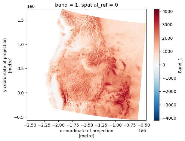

Success. Clearly, this DataArray contains information that allows matplotlib to create these “projection aware” axis labels. Or is matplotlib making some kind of assumption due to the non-rectangular nature of the data values? Hold that thought.

from pyproj import CRS

crs_102008 = CRS(dem_102008_xr.rio.crs)
crs_102008.axis_info

[Axis(name=Easting, abbrev=, direction=east, unit_auth_code=EPSG, unit_code=9001, unit_name=metre),
 Axis(name=Northing, abbrev=, direction=north, unit_auth_code=EPSG, unit_code=9001, unit_name=metre)]

During the process of figuring all this out, I frequently would have my Jupyter Lab kernel crash during reprojection related operations.

This led me to explore other options such as:

• using the GDAL executable program gdalwarp to do the reprojection using the underlying TIFF as the source and writing out a new TIFF,
• use the Python bindings to GDAL (from osgeo import gdal) to use gdal.warp - see https://gis.stackexchange.com/questions/233589/re-project-raster-in-python-using-gdal,

With respect to the Python bindings, I wasn’t sure if this was any different than using rioxarray as I was guessing that under the hood, both of these approaches were still using Python to access GDAL. Also, it’s highly suggested to not import gdal and rasterio in the same notebook session.

Reprojecting and resampling with GDAL command line utilities

As I describe here, GDAL is an indispensable part of computational geospatial work. In its set of command line utilities you can find gdalwarp which facilitates resampling, reprojection and even clipping. I found this set of notes that introduces GDAL along with Python.

Let’s create some variables for our input and output filenames.

dem_file = Path(WSFR_DATA_ROOT, 'hydrosheds/na_con_3s/na_con_3s.tif')
dem_file_102008_gdalwarp = Path(WSFR_DATA_ROOT, 'hydrosheds/na_con_3s/na_con_3s_102008_gdalwarp.tif')

Recall that we’ve got a bounding box specified in longitude and latitude.

print(extent_epsg_4326)

[-126, 35, -103, 52]

Here are the arguments used for gdalwarp:

• -t_srs ESRI:102008 - spatial reference system for the target.
• ts 2760 2040 - width and height in pixels for the target,
• -r bilinear - resampling method
• -te -126 35 -103 52 - the extent for the destination file. The default is to use the target spatial reference system, but…
• -te_srs EPSG:4326 - you can specify the spatial reference system used to define the extent.
• -dstnodata -9999 - specify the no data value in the target file.

gdalwarp_resample_cmd = f'gdalwarp -overwrite -t_srs ESRI:102008 -srcnodata 32767 -dstnodata -9999 -r bilinear -ts {dem_102008_xr.shape[2]} {dem_102008_xr.shape[1]} -te {minx_4326} {miny_4326} {maxx_4326} {maxy_4326} -te_srs EPSG:4326 {dem_file} {dem_file_102008_gdalwarp}'
!{gdalwarp_resample_cmd}

Creating output file that is 2760P x 2040L.
Processing /home/mark/Documents/projects/driven_data/wsfrodeo/data/hydrosheds/na_con_3s/na_con_3s.tif [1/1] : 0...10...20...30...40...50...60...70...80...90...100 - done.

Now read in the resampled and clipped GeoTIFF. We can use the masked=True option to convert the no data values to NaN.

dem_102008_gdalwarp_xr = rioxarray.open_rasterio(Path(dem_file_102008_gdalwarp), masked=True)

dem_102008_gdalwarp_xr

<xarray.DataArray (band: 1, y: 2040, x: 2760)>
[5630400 values with dtype=float32]
Coordinates:
  * band         (band) int64 1
  * x            (x) float64 -2.554e+06 -2.553e+06 ... -4.589e+05 -4.582e+05
  * y            (y) float64 1.431e+06 1.43e+06 ... -1.789e+05 -1.797e+05
    spatial_ref  int64 0
Attributes:
    AREA_OR_POINT:       Area
    RepresentationType:  THEMATIC
    scale_factor:        1.0
    add_offset:          0.0
    long_name:           Band_1

xarray.DataArray

• band: 1
• y: 2040
• x: 2760

• ...

  [5630400 values with dtype=float32]

• Coordinates: (4)
  • band
    (band)
    int64
    1

    array([1])

  • x
    (x)
    float64
    -2.554e+06 ... -4.582e+05

    array([-2553828.679341, -2553069.114766, -2552309.550191, ...,  -459709.146456,
            -458949.581881,  -458190.017307])

  • y
    (y)
    float64
    1.431e+06 1.43e+06 ... -1.797e+05

    array([1430769.171373, 1429979.350551, 1429189.52973 , ..., -178095.842566,
           -178885.663388, -179675.484209])

  • spatial_ref
    ()
    int64
    0

    crs_wkt :

    PROJCS["North_America_Albers_Equal_Area_Conic",GEOGCS["NAD83",DATUM["North_American_Datum_1983",SPHEROID["GRS 1980",6378137,298.257222101004,AUTHORITY["EPSG","7019"]],AUTHORITY["EPSG","6269"]],PRIMEM["Greenwich",0],UNIT["degree",0.0174532925199433,AUTHORITY["EPSG","9122"]],AUTHORITY["EPSG","4269"]],PROJECTION["Albers_Conic_Equal_Area"],PARAMETER["latitude_of_center",40],PARAMETER["longitude_of_center",-96],PARAMETER["standard_parallel_1",20],PARAMETER["standard_parallel_2",60],PARAMETER["false_easting",0],PARAMETER["false_northing",0],UNIT["metre",1,AUTHORITY["EPSG","9001"]],AXIS["Easting",EAST],AXIS["Northing",NORTH]]

    semi_major_axis :

    6378137.0

    semi_minor_axis :

    6356752.314140356

    inverse_flattening :

    298.257222101004

    reference_ellipsoid_name :

    GRS 1980

    longitude_of_prime_meridian :

    0.0

    prime_meridian_name :

    Greenwich

    geographic_crs_name :

    NAD83

    horizontal_datum_name :

    North American Datum 1983

    projected_crs_name :

    North_America_Albers_Equal_Area_Conic

    grid_mapping_name :

    albers_conical_equal_area

    standard_parallel :

    (20.0, 60.0)

    latitude_of_projection_origin :

    40.0

    longitude_of_central_meridian :

    -96.0

    false_easting :

    0.0

    false_northing :

    0.0

    spatial_ref :

    PROJCS["North_America_Albers_Equal_Area_Conic",GEOGCS["NAD83",DATUM["North_American_Datum_1983",SPHEROID["GRS 1980",6378137,298.257222101004,AUTHORITY["EPSG","7019"]],AUTHORITY["EPSG","6269"]],PRIMEM["Greenwich",0],UNIT["degree",0.0174532925199433,AUTHORITY["EPSG","9122"]],AUTHORITY["EPSG","4269"]],PROJECTION["Albers_Conic_Equal_Area"],PARAMETER["latitude_of_center",40],PARAMETER["longitude_of_center",-96],PARAMETER["standard_parallel_1",20],PARAMETER["standard_parallel_2",60],PARAMETER["false_easting",0],PARAMETER["false_northing",0],UNIT["metre",1,AUTHORITY["EPSG","9001"]],AXIS["Easting",EAST],AXIS["Northing",NORTH]]

    GeoTransform :

    -2554208.4616283667 759.5645748584358 0.0 1431164.0817839599 0.0 -789.8208217668104

    array(0)

• Indexes: (3)
  • band
    PandasIndex

    PandasIndex(Index([1], dtype='int64', name='band'))

  • x
    PandasIndex

    PandasIndex(Index([-2553828.6793409376,  -2553069.114766079,  -2552309.550191221,
            -2551549.985616362,  -2550790.421041504, -2550030.8564666454,
            -2549271.291891787, -2548511.7273169286,   -2547752.16274207,
           -2546992.5981672117,
           ...
            -465026.0984802393,  -464266.5339053809, -463506.96933052246,
           -462747.40475566406,  -461987.8401808054,   -461228.275605947,
            -460468.7110310886,  -459709.1464562302,  -458949.5818813718,
            -458190.0173065134],
          dtype='float64', name='x', length=2760))

  • y
    PandasIndex

    PandasIndex(Index([ 1430769.1713730765,  1429979.3505513098,  1429189.5297295428,
             1428399.708907776,  1427609.8880860093,  1426820.0672642426,
            1426030.2464424756,  1425240.4256207088,   1424450.604798942,
            1423660.7839771751,
           ...
            -172567.0968135486, -173356.91763531533, -174146.73845708207,
           -174936.55927884905,  -175726.3801006158, -176516.20092238253,
           -177306.02174414927, -178095.84256591625,   -178885.663387683,
           -179675.48420944973],
          dtype='float64', name='y', length=2040))

• Attributes: (5)

  AREA_OR_POINT :

  Area

  RepresentationType :

  THEMATIC

  scale_factor :

  1.0

  add_offset :

  0.0

  long_name :

  Band_1

dem_102008_gdalwarp_xr[0][0:10][0:10].values

array([[ nan,  nan,  nan, ..., 609., 609., 609.],
       [ nan,  nan,  nan, ..., 608., 607., 606.],
       [ nan,  nan,  nan, ..., 607., 606., 605.],
       ...,
       [ nan,  nan,  nan, ..., 601., 599., 595.],
       [ nan,  nan,  nan, ..., 598., 596., 593.],
       [ nan,  nan,  nan, ..., 595., 593., 590.]], dtype=float32)

Clearly this is different than the values in dem_102008_xr. It seems like rio.reproject is behaving differently than gdalwarp.

# Summary stats of new resample raster
print(f'crs: {dem_102008_gdalwarp_xr.rio.crs}')
print(f'bounds: {dem_102008_gdalwarp_xr.rio.bounds()}')
print(f'shape: {dem_102008_gdalwarp_xr.shape}')
print(f'Number of cells: {dem_102008_gdalwarp_xr.shape[1] * dem_102008_gdalwarp_xr.shape[2]:,}')
print(f'Number of data cells: {(~dem_102008_gdalwarp_xr.isnull()).values.sum():,}')
print(f'nodata value: {dem_102008_gdalwarp_xr.rio.nodata}')
print(f'original nodata value: {dem_102008_gdalwarp_xr.rio.encoded_nodata}')

crs: ESRI:102008
bounds: (-2554208.4616283667, -180070.39462033313, -457810.2350190842, 1431164.0817839599)
shape: (1, 2040, 2760)
Number of cells: 5,630,400
Number of data cells: 4,421,827
nodata value: nan
original nodata value: -9999.0

So, there are many more data values in this raster than there are in dem_102008_xr. Obviously the bounds are different (not sure why they are different) but that in and of itself shouldn’t affect the invidual pixel values within the bounds, or does it?

dem_102008_gdalwarp_xr.plot()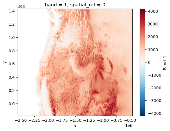

Why does this look different than the raster plotted based on the reprojection done with rio.reproject? The rasters are the same shape and have the same CRS. But the bounds are different, individual data values are different for some pixels and the resulting plots are different - the one based on the gdalwarp raster has standard x and y coordinates.

CRS(dem_102008_gdalwarp_xr.rio.crs).axis_info

[Axis(name=Easting, abbrev=, direction=east, unit_auth_code=EPSG, unit_code=9001, unit_name=metre),
 Axis(name=Northing, abbrev=, direction=north, unit_auth_code=EPSG, unit_code=9001, unit_name=metre)]

Let’s make sure they both have the same CRS.

if dem_102008_xr.rio.crs == dem_102008_gdalwarp_xr.rio.crs:
    print(f'Both have CRS = {dem_102008_xr.rio.crs}')
else:
    printf(f'rioxarray CRS: {dem_102008_xr.rio.crs}\ngdalwarp CRS: {dem_102008_gdalwarp_xr.rio.crs}')

Both have CRS = ESRI:102008

So, it doesn’t seem to have anything to do with the projection differences.

print(f'resolution: {dem_102008_xr.rio.resolution()}')
print(f'gdalwarp  : {dem_102008_gdalwarp_xr.rio.resolution()}')

resolution: (759.5870288351857, -1121.4450217146702)
gdalwarp  : (759.5645748584358, -789.8208217668104)

Pixel height differs.

print(dem_102008_xr.attrs)
print(dem_102008_gdalwarp_xr.attrs)

{'AREA_OR_POINT': 'Area', 'RepresentationType': 'THEMATIC', 'scale_factor': 1.0, 'add_offset': 0.0, 'long_name': 'Band_1'}
{'AREA_OR_POINT': 'Area', 'RepresentationType': 'THEMATIC', 'scale_factor': 1.0, 'add_offset': 0.0, 'long_name': 'Band_1'}

print(dem_102008_xr.rio.grid_mapping)
print(dem_102008_gdalwarp_xr.rio.grid_mapping)

spatial_ref
spatial_ref

Let’s check the affine transform that was used for each of these.

print('transform\n',dem_102008_xr.rio.transform(),'\n')
print('_cached_transform\n',dem_102008_xr.rio._cached_transform(), '\n')
print('recalced transform\n', dem_102008_xr.rio.transform(recalc=True))

transform
 | 759.59, 0.00,-2554208.46|
| 0.00,-1121.45, 1722498.45|
| 0.00, 0.00, 1.00| 

_cached_transform
 | 759.59, 0.00,-2554208.46|
| 0.00,-1121.45, 1722498.45|
| 0.00, 0.00, 1.00| 

recalced transform
 | 759.59, 0.00,-2554208.46|
| 0.00,-1121.45, 1722498.45|
| 0.00, 0.00, 1.00|

print('transform\n',dem_102008_gdalwarp_xr.rio.transform(),'\n')
print('_cached_transform\n',dem_102008_gdalwarp_xr.rio._cached_transform(),'\n')
print('recalced transform\n',dem_102008_gdalwarp_xr.rio.transform(recalc=True))

transform
 | 759.56, 0.00,-2554208.46|
| 0.00,-789.82, 1431164.08|
| 0.00, 0.00, 1.00| 

_cached_transform
 | 759.56, 0.00,-2554208.46|
| 0.00,-789.82, 1431164.08|
| 0.00, 0.00, 1.00| 

recalced transform
 | 759.56, 0.00,-2554208.46|
| 0.00,-789.82, 1431164.08|
| 0.00, 0.00, 1.00|

Ok, there’s another difference. Time to learn more about the transforms. The transform matrices are used to make affine transformations between rasters and CRS. This post explains affine transformations in the context of using Python for GIS work.

The elements of the above matrices are:

\[ \begin{bmatrix} a & b & c\\ d & e & f\\ g & h & i \end{bmatrix} \]

where

• \(a\) - width of a pixel
• \(b\) - row rotation (typically 0)
• \(c\) - x-coordinate of upper left corner of upper left pixel
• \(d\) - column rotation (typically 0)
• \(e\) - height of a pixel (typicaly negative)
• \(f\) - y-coordinate of upper left corner of upper left pixel

The \(g=0\), \(h=0\), and \(i=1\) entries are constants.

It’s the second row of the matrices for dem_102008_xr and dem_102008_gdalwarp_xr that differ by a large amount. The pixel size and y-coordinates are really quite different for the two matrices.

• dem_102008_xr - | 0.00,-1121.45, 1722498.45|
• dem_102008_gdalwarp_xr - | 0.00,-789.82, 1431164.08|

Both rasters have 2040 rows.

print(f'bounds:\t\t {dem_102008_xr.rio.bounds()}')
print(f'gdalbounds:\t {dem_102008_gdalwarp_xr.rio.bounds()}')

bounds:      (-2554208.4616283686, -565249.3965455483, -457748.2620432562, 1722498.447752379)
gdalbounds:  (-2554208.4616283667, -180070.39462033313, -457810.2350190842, 1431164.0817839599)

We should be able to match the bounds using pixel height and the number of rows.

# rioxarray version
2040 * -1121.45 + 1722498.45

-565259.55

# gdalwarp version
2040 * -789.82 + 1431164.08

-180068.71999999997

Yep, the relationship between the pixel height and the bounds in the y-dimension are as expected.

So, the question is, why does rio.reproject and gdalwarp using different affine transformations for what seems like the same reprojection to ESRI:102008 with the same shape?

It appears from these two sources that GDAL/PROJ make the choice from among possibly multiple suitable transformations:

• https://gis.stackexchange.com/questions/441871/return-used-transformation-from-gdal-warp-or-similar
• https://gdal.org/tutorials/osr_api_tut.html

It seems like the -ct argument in gdalwarp can be used to specify a PROJ or WKT2 string that forces a specific transformation to be used.

You can see what PROJ is doing by running this at the command line.

projinfo -s epsg:4326 -t esri:102008

Similar issues related to differences between projections done with rioxarray and gdalwarp include:

• https://github.com/rasterio/rasterio/issues/2052
• https://github.com/rasterio/rasterio/issues/1990

Okay, we’ll just leave this issue here for now.

A little more reprojection exploration

As part of trying to understand the various ways of getting the reprojection done, I tried to explore things in a bit greater detail. For example, what was the relationship between the bounds reported by rio.bounds and the actual values in the xarray DataArray?

gdal_bounds = dem_102008_gdalwarp_xr.rio.bounds()
gdal_bounds

(-2554208.4616283667,
 -180070.39462033313,
 -457810.2350190842,
 1431164.0817839599)

minx_gdal = dem_102008_gdalwarp_xr['x'].values.min()
maxx_gdal = dem_102008_gdalwarp_xr['x'].values.max()
miny_gdal = dem_102008_gdalwarp_xr['y'].values.min()
maxy_gdal = dem_102008_gdalwarp_xr['y'].values.max()

print(f"minx: {minx_gdal}")
print(f"maxx: {maxx_gdal}")

print(f"miny: {miny_gdal}")
print(f"maxy: {maxy_gdal}")

minx: -2553828.6793409376
maxx: -458190.0173065134
miny: -179675.48420944973
maxy: 1430769.1713730765

print(f"minx diff: {ureg.Quantity(gdal_bounds[0] - minx_gdal, 'meters')}") 
print(f"miny diff: {ureg.Quantity(gdal_bounds[1] - miny_gdal, 'meters')}") 

print(f"maxx diff: {ureg.Quantity(gdal_bounds[2] - maxx_gdal, 'meters')}") 
print(f"maxy diff: {ureg.Quantity(gdal_bounds[3] - maxy_gdal, 'meters')}") 

minx diff: -379.78228742908686 meter
miny diff: -394.9104108833999 meter
maxx diff: 379.7822874292033 meter
maxy diff: 394.9104108833708 meter

The difference between the bounds as reported by rioxarray and the minimums and maximums based on the values of the appropriate dimensions in the underlying xarray DataArray are half of the corresponding x and y pixel sizes. So, rio.bounds is the edge of the pixels and values must be the midpoint of the pixels. Makes sense.

Creating maps with Cartopy

One method for creating maps in Python has been the Basemap toolkit which is part of matplotlib. This has now been deprecated in favor of the Cartopy project. So, that’s what we’ll use.

From the Cartopy docs:

• Cartopy is a Python package designed for geospatial data processing in order to produce maps and other geospatial data analyses.

• Cartopy makes use of the powerful PROJ, NumPy and Shapely libraries and includes a programmatic interface built on top of Matplotlib for the creation of publication quality maps.

• Key features of cartopy are its object oriented projection definitions, and its ability to transform points, lines, vectors, polygons and images between those projections.

• You will find cartopy especially useful for large area / small scale data, where Cartesian assumptions of spherical data traditionally break down. If you’ve ever experienced a singularity at the pole or a cut-off at the dateline, it is likely you will appreciate cartopy’s unique features!

Projections in Cartopy

Cartopy provides an object oriented way to work with map projections through its cartopy.crs.CRS class. We need to import the cartopy.crs module.

import cartopy.crs as ccrs                   # import projections

Let’s create a CRS object for the Albers Equal Area projection that we’ll use for the map. Set the central lat/lon and standard parallels to something that makes sense for the region being mapped. I’m going to specify these parameters explicitly even though they are the default values.

crs_aea = ccrs.AlbersEqualArea(central_longitude=-96,
                               central_latitude=40,
                               standard_parallels=(20.0, 60.0))

Basic cartopy plot

For the map, we’ll experiment with using map extents based on both of the DEM rasters we created.

minx_102008_gdalwarp, maxx_102008_gdalwarp, miny_102008_gdalwarp, maxy_102008_gdalwarp = \
    dem_102008_gdalwarp_xr.rio.bounds()

The order of these bounds in Cartopy’s set_extent() function is different than the order in the bounds as reported by rioxarray. Cartopy uses (minx, maxx, miny, maxy).

cartopy_extent_102008_gdalwarp = (minx_102008_gdalwarp, maxx_102008_gdalwarp, miny_102008_gdalwarp, maxy_102008_gdalwarp)
cartopy_extent_102008 = (minx_102008, maxx_102008, miny_102008, maxy_102008)

We start with standard matplotlib figure creation.

# Create figure and set size
fig1 = plt.figure()
fig1.set_figheight(9)
fig1.set_figwidth(16)

<Figure size 1600x900 with 0 Axes>

Cartopy contains a GeoAxes class built on top of the regular matplotlib Axes class and embues with geospatial powers. When creating such an Axes object, you need to pass in the CRS.

Next we can set the map extent with GeoAxes.set_extent(). We’ll start with the extent based on the raster reprojected with rioxarray.

Then, add_geometries method is used to add the vector layers to the GeoAxes instance. One gotcha is that this method doesn’t seem to work correctly with points. To get around this, we can simply use the plot method in GeoPandas (which is also based on matplotlib).

Similarly, we can use the plot method from xarray and rioxarray to add the DEM raster to the plot.

# Create figure and set size
fig1 = plt.figure()
fig1.set_figheight(9)
fig1.set_figwidth(16)

# create a set of axes with desired projection  
ax1 = plt.axes(projection = crs_aea)

# Set map extent
ax1.set_extent(cartopy_extent_102008, crs = crs_aea)

# Add sites and basins
ax1.add_geometries(basins_102008_gdf.geometry, crs=crs_aea, facecolor="#a2d572", edgecolor="grey", linewidth=0.5) # for Lat/Lon data.
sites_102008_gdf.plot(ax=ax1, marker="D") # add_geometries doesn't seem to work with points

# Add state and province boundaries
ax1.add_geometries(state_102008_gdf.geometry, crs = crs_aea, facecolor="none", edgecolor="black", linewidth=0.3)
ax1.add_geometries(province_102008_gdf.geometry, crs = crs_aea, facecolor="none", edgecolor="black", linewidth=0.3)

# Add rivers
ax1.add_geometries(rivers_102008_gdf.geometry, crs = crs_aea, edgecolor="#487bb6", linewidth=0.75)

# Add DEM raster
dem_102008_xr.plot(ax=ax1, cmap='terrain')

ax1.set_title("Map 1 - using DEM and extent from rioxarray processed raster")                    
plt.show()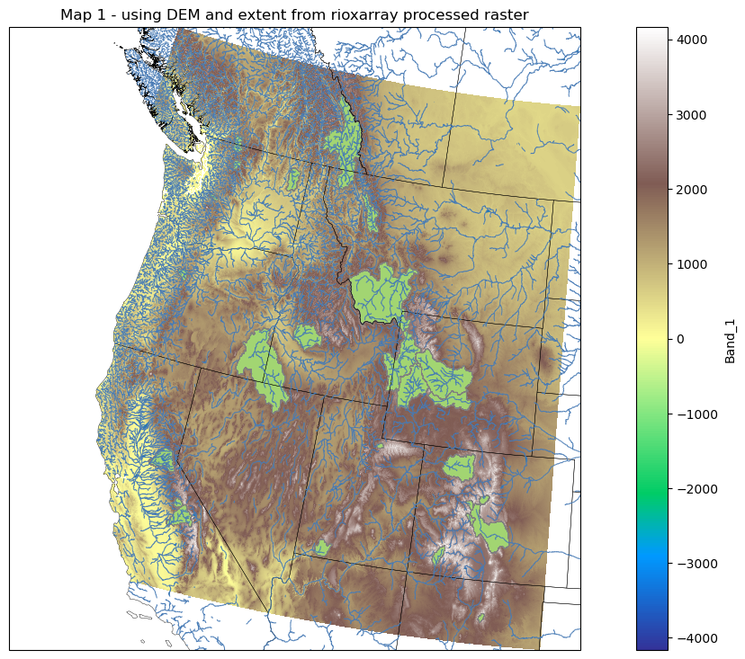

Hmm, the way that rioxarray did the projection resulted in numerous no data values within the extent of the map. At this point, I don’t completely understand what is going on. What happens if we use the extent and raster based on gdalwarp?

# Create figure and set size
fig2 = plt.figure()
fig2.set_figheight(9)
fig2.set_figwidth(16)

# create a set of axes with desired projection  
ax2 = plt.axes(projection = crs_aea)  # create a set of axes with desired projection    

# Set map extent
ax2.set_extent(cartopy_extent_102008_gdalwarp, crs = crs_aea)

# Add sites and basins
ax2.add_geometries(basins_102008_gdf.geometry, crs=crs_aea, facecolor="#a2d572", edgecolor="grey", linewidth=0.5) # for Lat/Lon data.
sites_102008_gdf.plot(ax=ax2, marker="D") # add_geometries doesn't seem to work with points

# Add state and province boundaries
ax2.add_geometries(state_102008_gdf.geometry, crs = crs_aea, facecolor="none", edgecolor="black", linewidth=0.3)
ax2.add_geometries(province_102008_gdf.geometry, crs = crs_aea, facecolor="none", edgecolor="black", linewidth=0.3)

# Add rivers
ax2.add_geometries(rivers_102008_gdf.geometry, crs = crs_aea, edgecolor="#487bb6", linewidth=0.75)

# Add DEM raster
dem_102008_gdalwarp_xr.plot(ax=ax2, cmap='terrain')

ax2.set_title("Map 2 - using DEM and extent from gdalwarp processed raster")                    
plt.show()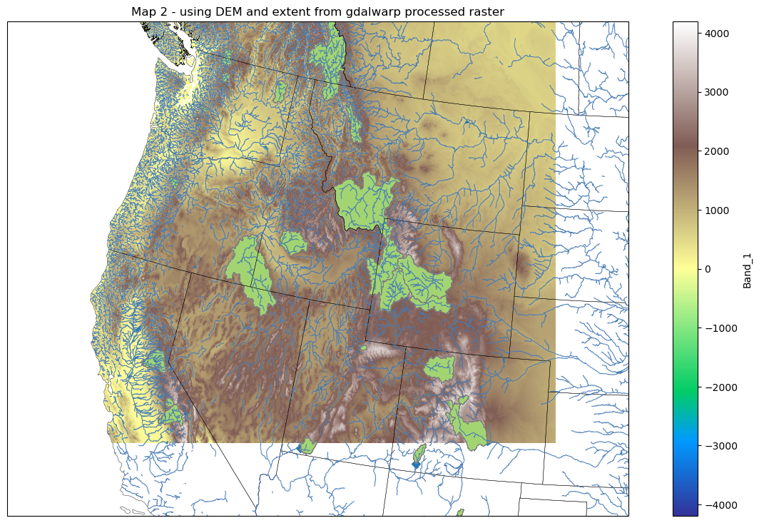

Now the raster doesn’t cover the entire map in the y-dimension. This is consistent with the affine transformation used by gdalwarp but certainly isn’t desirable. The original lat/lon bounds based on EPSG:4326 included all of the vector layers in their entirety. I’m a bit baffled by these reprojection and bounding box issues. It will have to be the topic of another post as I’ve wasted way too much time fighting with these problems.

Using built in and NaturalEarth features

Cartopy makes it easy to use preinstalled features such as state borders and rivers as well as those from the Natural Earth dataset through the cartopy.feature module. To do this we use the add_feature GeoAxes method. Standard matplotlib keyword arguments can be passed in as well to style the feature. Use the zorder parameter to control which layers are above and below other layers. Higher numbered layers are plotted on top of lower numbered layers.

import cartopy.feature as cf                 # import features

# Create a land feature to act as the basemap
land_50m = cf.NaturalEarthFeature('physical', 'land', '50m',
                                  edgecolor='k', facecolor="none", alpha=0.5)

fig = plt.figure()
fig.set_figheight(8)
fig.set_figwidth(12)

crs_aea = ccrs.AlbersEqualArea(central_longitude=-96,
                               central_latitude=40,
                               standard_parallels=(20.0, 60.0))

ax = plt.axes(projection = crs_aea)
ax.set_extent(cartopy_extent_102008, crs = crs_aea)

# Add features
ax.add_feature(land_50m, zorder=8, alpha=0.5)
ax.add_feature(cf.LAKES, zorder=3)
ax.add_feature(cf.OCEAN, zorder=4)
ax.add_feature(cf.BORDERS, zorder=6)
ax.add_feature(cf.COASTLINE, zorder=6)
ax.add_feature(cf.STATES, zorder=6)
ax.add_feature(cf.RIVERS, zorder=9)

# Add our vector layers
ax.add_geometries(basins_102008_gdf.geometry, crs = crs_aea, zorder=10,
                  facecolor="#a2d572", edgecolor="grey", linewidth=0.5) # for Lat/Lon data.
sites_102008_gdf.plot(ax=ax, marker="D")

# Add DEM raster
dem_102008_xr.plot(ax=ax, cmap='terrain')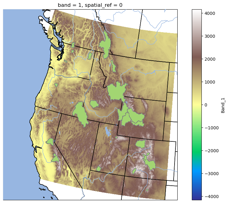

More Cartopy and other resources

• Cartography and mapping in Python
• Plotting Actual Things: geopandas and cartopy
• Maps in Scientific Python
• pyheds - Simple and fast watershed delineation in python
• Plotting raster and vector data together in python

More Python mapping tools

This post has barely scratched the surface of Python based mapping tools. We will explore other tools such as Folium and leafmap in subsequent posts.

• Folium - https://python-visualization.github.io/folium/latest/
• leafmap - https://leafmap.org/
• ipyleaflet - https://github.com/jupyter-widgets/ipyleaflet
• hvPlot - https://github.com/holoviz/hvplot
• Cartopy - https://github.com/SciTools/cartopy
• geoviews - https://github.com/holoviz/geoviews
• eomaps - https://github.com/raphaelquast/eomaps

Using R to create a river map

In Part 3 of this series we’ll take a look at using R to create a similar river map. For the R based map, I decided to create a separate post written with Quarto to avoid messing around with the r2py package within Jupyter notebooks.