import io
import os
from pathlib import Path

import pandas as pd
from IPython.display import ImageA vector-raster river map, three ways - Part 1: QGIS
and then we’ll repeat using Python and R
geonewb
geospatial
python
qgis
Creating a river map using QGIS, Python, and R
This is part of my geonewb series of posts.
I’m using the Water Supply Rodeo Forecast Challenge run by the Driven Data folks to further my geospatial analysis learning. This series of posts is going to focus on a basic step that was motivated by the challenge - create a map showing the relevant rivers and river basins. Such a map would combine several vector and raster datasets:
- a vector layer with the stream guage sites
- a vector layer with watershed basin boundaries
- a vector layer showing US state boundaries and Canadian province boundaries
- a vector layer showing rivers
- a raster layer containing a DEM
My goal is to create maps using three different technologies: QGIS, Python and R. By doing this I can get a sense of the open source mapping landscape at a beginner level. In this first post, we’ll use QGIS, a widely used open source GIS package. This is NOT a basic QGIS tutorial - there are plenty of those out there and the documentation is quite good.
WSFR_DATA_ROOT = os.environ['WSFR_DATA_ROOT']Here’s what one of the final QGIS maps looks like:
Image('./images/WaterSupplyForecastRodeo.png')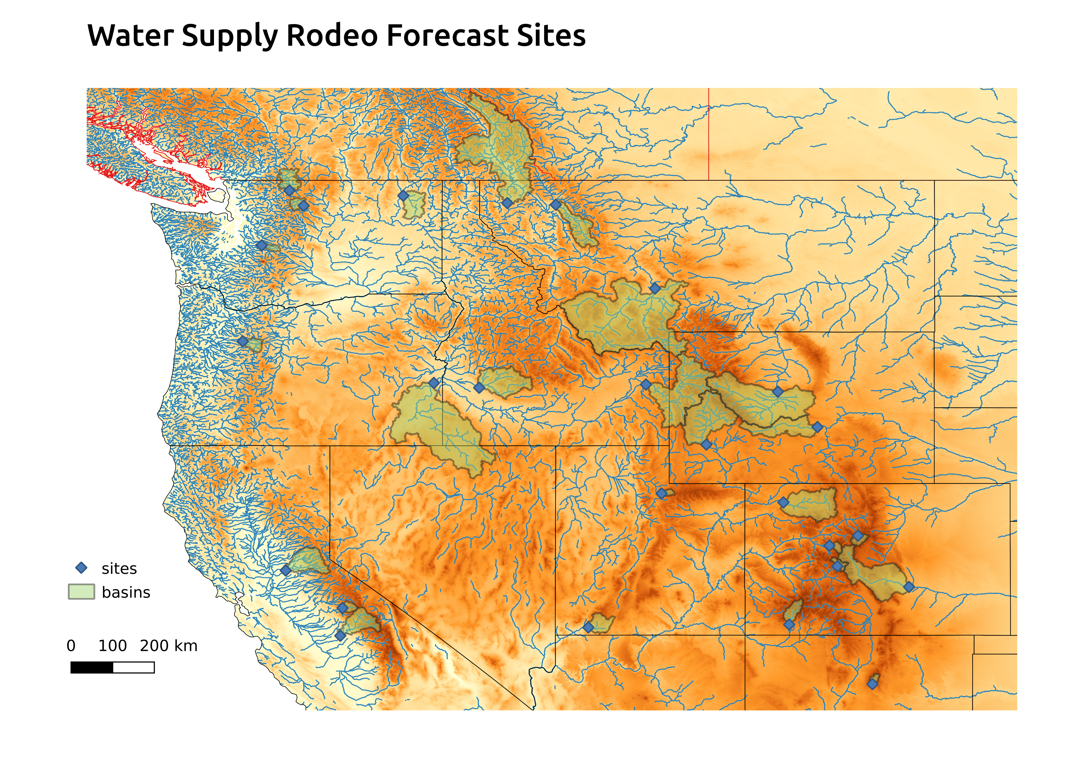
Data sources and Python libraries
All of the data we need is freely available. Even though this first map is created with QGIS, we will start to use some Python libraries to explore the data that we’ll be using. In particular, we will use the GeoPandas package to read vector data into GeoDataFrame objects. GeoPandas adds geospatial functionality to pandas.
GeoPandas is an open source project to make working with geospatial data in python easier. GeoPandas extends the datatypes used by pandas to allow spatial operations on geometric types. Geometric operations are performed by shapely. GeoPandas further depends on fiona for file access and matplotlib for plotting.
For raster data, we’ll use the xarray and rioxarray packages.
The xarray package builds on top of NumPy N-d arrays and adds ability to create and work with labels for the dimensions.
The two main data structures are DataArray (a N-d generalization of a pandas.Series) and DataSet (an N-d generalization of a pandas.DataFrame). The Overview: Why xarray? page has a nice level of detail on the case for xarray and its link to geospatial analysis.
The rioxarray package extends the xarray package to facilitate reading raster data into xarray objects. The actual reading of the raster file is done using another Python package, rasterio. From the rasterio docs:
Geographic information systems use GeoTIFF and other formats to organize and store gridded raster datasets such as satellite imagery and terrain models. Rasterio reads and writes these formats and provides a Python API based on Numpy N-dimensional arrays and GeoJSON.
Sites and basins (vector)
The streamflow guage sites and associated watershed basins are defined in the geospatial.gpkg GeoPackage file available from the WSFR data downloads page. GeoPackage files can contain multiple layers of both vector and raster data. Individual layers can be read using GeoPandas’ read_file method by passing the layer name. The layer= argument is actually passed along to Fiona, a Python wrapper for accessing vector data via the GDAL/OGR library.
Under the hood, a GeoPackage is a SQLite database that conforms to the GeoPackage standard developed by the Open Geospatial Consortium. Both basins and sites are tables in the GeoPackage (SQLite database) and can be accessed directly with a SQLite database browser or any tool for working with SQLite databases. If you omit the layer= argument, GeoPandas returns the basins layer, likely as it’s the first layer in whatever internal indexing scheme is used with the collection of layers.
import geopandas as gpd

# Reading a GeoPackage file
geospatial_input_file = Path(WSFR_DATA_ROOT, 'geospatial.gpkg')
basins_gdf = gpd.read_file(geospatial_input_file, layer='basins')
sites_gdf = gpd.read_file(geospatial_input_file, layer='sites')basins_gdf| site_id | name | area | geometry | |
|---|---|---|---|---|
| 0 | hungry_horse_reservoir_inflow | Hungry Horse Reservoir Inflow | 1681.780 | POLYGON ((-113.09701 47.24399, -113.09730 47.2... |
| 1 | snake_r_nr_heise | Snake River near Heise | 5719.410 | MULTIPOLYGON (((-110.79196 44.40127, -110.7922... |
| 2 | pueblo_reservoir_inflow | Pueblo Reservoir Inflow | 4615.460 | POLYGON ((-105.67340 38.15883, -105.67315 38.1... |
| 3 | sweetwater_r_nr_alcova | Sweetwater River near Alcova | 2377.280 | POLYGON ((-107.32822 42.21621, -107.32903 42.2... |
| 4 | missouri_r_at_toston | Missouri River at Toston | 14676.200 | POLYGON ((-110.63001 46.30856, -110.63006 46.3... |
| 5 | animas_r_at_durango | Animas River at Durango | 700.901 | POLYGON ((-107.87584 37.27614, -107.87759 37.2... |
| 6 | yampa_r_nr_maybell | Yampa River near Maybell | 3381.680 | MULTIPOLYGON (((-107.02802 40.02615, -107.0277... |
| 7 | libby_reservoir_inflow | Libby Reservoir Inflow | 9030.450 | MULTIPOLYGON (((-114.85817 48.50961, -114.8582... |
| 8 | boise_r_nr_boise | Boise River near Boise | 2687.340 | MULTIPOLYGON (((-115.23528 44.09596, -115.2355... |
| 9 | green_r_bl_howard_a_hanson_dam | Green River below Howard Hanson Dam | 221.234 | POLYGON ((-121.31474 47.13373, -121.31530 47.1... |
| 10 | taylor_park_reservoir_inflow | Taylor Park Reservoir Inflow | 254.415 | MULTIPOLYGON (((-106.74944 39.04268, -106.7499... |
| 11 | dillon_reservoir_inflow | Dillon Reservoir Inflow | 328.429 | POLYGON ((-106.04383 39.35748, -106.04564 39.3... |
| 12 | ruedi_reservoir_inflow | Ruedi Reservoir Inflow | 223.740 | POLYGON ((-106.52087 39.15795, -106.52216 39.1... |
| 13 | fontenelle_reservoir_inflow | Fontenelle Reservoir Inflow | 4199.150 | POLYGON ((-110.06865 42.02568, -110.06944 42.0... |
| 14 | weber_r_nr_oakley | Weber River near Oakley | 162.429 | POLYGON ((-111.06529 40.67623, -111.06633 40.6... |
| 15 | san_joaquin_river_millerton_reservoir | San Joaquin River - Millerton Reservoir | 1886.720 | MULTIPOLYGON (((-120.44227 39.29433, -120.4423... |
| 16 | merced_river_yosemite_at_pohono_bridge | Merced River - Yosemite at Pohono Bridge | 321.858 | POLYGON ((-119.44368 37.86102, -119.44401 37.8... |
| 17 | american_river_folsom_lake | American River - Folsom Reservoir | 1677.530 | MULTIPOLYGON (((-119.52661 37.04015, -119.5265... |
| 18 | colville_r_at_kettle_falls | Colville River at Kettle Falls | 1086.250 | POLYGON ((-117.88747 48.70666, -117.88776 48.7... |
| 19 | stehekin_r_at_stehekin | Stehekin River at Stehekin | 319.664 | POLYGON ((-120.93255 48.19748, -120.93284 48.1... |
| 20 | detroit_lake_inflow | Detroit Lake Inflow | 452.383 | POLYGON ((-121.85271 44.46766, -121.85379 44.4... |
| 21 | virgin_r_at_virtin | Virgin River at Virgin | 948.039 | MULTIPOLYGON (((-112.73274 37.06034, -112.7327... |
| 22 | skagit_ross_reservoir | Ross Reservoir Inflow | 800.749 | MULTIPOLYGON (((-120.98078 48.74358, -120.9810... |
| 23 | boysen_reservoir_inflow | Boysen Reservoir Inflow | 7706.580 | POLYGON ((-108.50590 42.46772, -108.50643 42.4... |
| 24 | pecos_r_nr_pecos | Pecos River near Pecos | 171.839 | MULTIPOLYGON (((-105.50099 35.90638, -105.5007... |
| 25 | owyhee_r_bl_owyhee_dam | Owyhee River below Owyhee Dam | 11659.800 | POLYGON ((-118.19040 43.09658, -118.19034 43.0... |
sites_gdf| site_id | name | geometry | |
|---|---|---|---|
| 0 | hungry_horse_reservoir_inflow | Hungry Horse Reservoir Inflow | POINT (-114.03786 48.35658) |
| 1 | snake_r_nr_heise | Snake River near Heise | POINT (-111.66000 43.61250) |
| 2 | pueblo_reservoir_inflow | Pueblo Reservoir Inflow | POINT (-104.71803 38.27167) |
| 3 | sweetwater_r_nr_alcova | Sweetwater River near Alcova | POINT (-107.13394 42.48996) |
| 4 | missouri_r_at_toston | Missouri River at Toston | POINT (-111.42028 46.14657) |
| 5 | animas_r_at_durango | Animas River at Durango | POINT (-107.88035 37.27917) |
| 6 | yampa_r_nr_maybell | Yampa River near Maybell | POINT (-108.03341 40.50275) |
| 7 | libby_reservoir_inflow | Libby Reservoir Inflow | POINT (-115.31872 48.40066) |
| 8 | boise_r_nr_boise | Boise River near Boise | POINT (-116.05955 43.52767) |
| 9 | green_r_bl_howard_a_hanson_dam | Green River below Howard Hanson Dam | POINT (-121.79789 47.28371) |
| 10 | taylor_park_reservoir_inflow | Taylor Park Reservoir Inflow | POINT (-106.60920 38.81833) |
| 11 | dillon_reservoir_inflow | Dillon Reservoir Inflow | POINT (-106.06641 39.62554) |
| 12 | ruedi_reservoir_inflow | Ruedi Reservoir Inflow | POINT (-106.81865 39.36387) |
| 13 | fontenelle_reservoir_inflow | Fontenelle Reservoir Inflow | POINT (-110.06667 42.02778) |
| 14 | weber_r_nr_oakley | Weber River near Oakley | POINT (-111.24796 40.73717) |
| 15 | san_joaquin_river_millerton_reservoir | San Joaquin River - Millerton Reservoir | POINT (-119.72431 36.98439) |
| 16 | merced_river_yosemite_at_pohono_bridge | Merced River - Yosemite at Pohono Bridge | POINT (-119.66567 37.71628) |
| 17 | american_river_folsom_lake | American River - Folsom Reservoir | POINT (-121.16436 38.70453) |
| 18 | colville_r_at_kettle_falls | Colville River at Kettle Falls | POINT (-118.06249 48.59435) |
| 19 | stehekin_r_at_stehekin | Stehekin River at Stehekin | POINT (-120.69177 48.32958) |
| 20 | detroit_lake_inflow | Detroit Lake Inflow | POINT (-122.29744 44.75378) |
| 21 | virgin_r_at_virtin | Virgin River at Virgin | POINT (-113.18078 37.20415) |
| 22 | skagit_ross_reservoir | Ross Reservoir Inflow | POINT (-121.06761 48.73217) |
| 23 | boysen_reservoir_inflow | Boysen Reservoir Inflow | POINT (-108.17899 43.42496) |
| 24 | pecos_r_nr_pecos | Pecos River near Pecos | POINT (-105.68270 35.70835) |
| 25 | owyhee_r_bl_owyhee_dam | Owyhee River below Owyhee Dam | POINT (-117.25583 43.65444) |
State and provincial boundaries (vector)
The US government provides Cartographic Boundary Files in both geodatabase and shapefile formats. They are available at different levels of resolution and also by geographic region.
The cartographic boundary files are simplified representations of selected geographic areas from the Census Bureau’s Master Address File/Topologically Integrated Geographic Encoding and Referencing (MAF/TIGER) System. These boundary files are specifically designed for small scale thematic mapping. As of 2019, cartographic boundary files are available in shapefile, geodatabase, and Keyhole Markup Language (KML) format. For more details about these files, including their appropriate usage, please see our Cartographic Boundary File Description page.
I downloaded the lowest resolution (1:20,000,000) zipped geodatabase file of the entire US. Uncompressing it results in a folder that is the geodatabase.
Since some of the basins are in Canada, I found similar maps for Canada in shapefile format.
River layer (vector)
For this layer we can use HydroRIVERS data, a part of the HydroSHEDS project. Both geodatase and shapefile formats are downloadable from https://www.hydrosheds.org/products/hydrorivers. There are different files for different regions of the world. The North American and Central America data as a zipped geodatabase is available from here and is ~72Mb in size (compressed). Unzip it after downloading. It’s a lot of rivers.
DEM layer (raster)
Since this project is all about hydrology, we will use a specially “hydrologically conditioned DEM” available as part of the HydroSHEDS core layer.
- go to https://www.hydrosheds.org/hydrosheds-core-downloads,
- select the Conditioned DEM tab near bottom of page,
- download the compressed file for North and Central America; it’s ~2.7GB,
- uncompress the downloaded file and you’ll get a folder containing documentation and the GeoTIFF file,
na_con_3s.tif, with the DEM raster.
Using QGIS to create the map
QGIS is a widely used, free and open source, GIS package. Check out the documentation.
The main steps we’ll do are:
- Create a new project
- Connect to the geospatial.gpkg file using the Data Source Manager and add the sites (points) and basins (polygons) layers.
- Add the state and province boundaries from a geodatabase and shapefile, respectively.
- Add the DEM layer from a GeoTIFF file.
- Add the rivers from a geodatabase.
- Make styling changes and create a print layout.
Adding the sites and basins
Use the Data Source Manager to connect to the geospatial.gpkg file and select the sites and basins layers to add to the map. After doing that, the map looks like this.
Image('./images/qgis_sites_basins.png')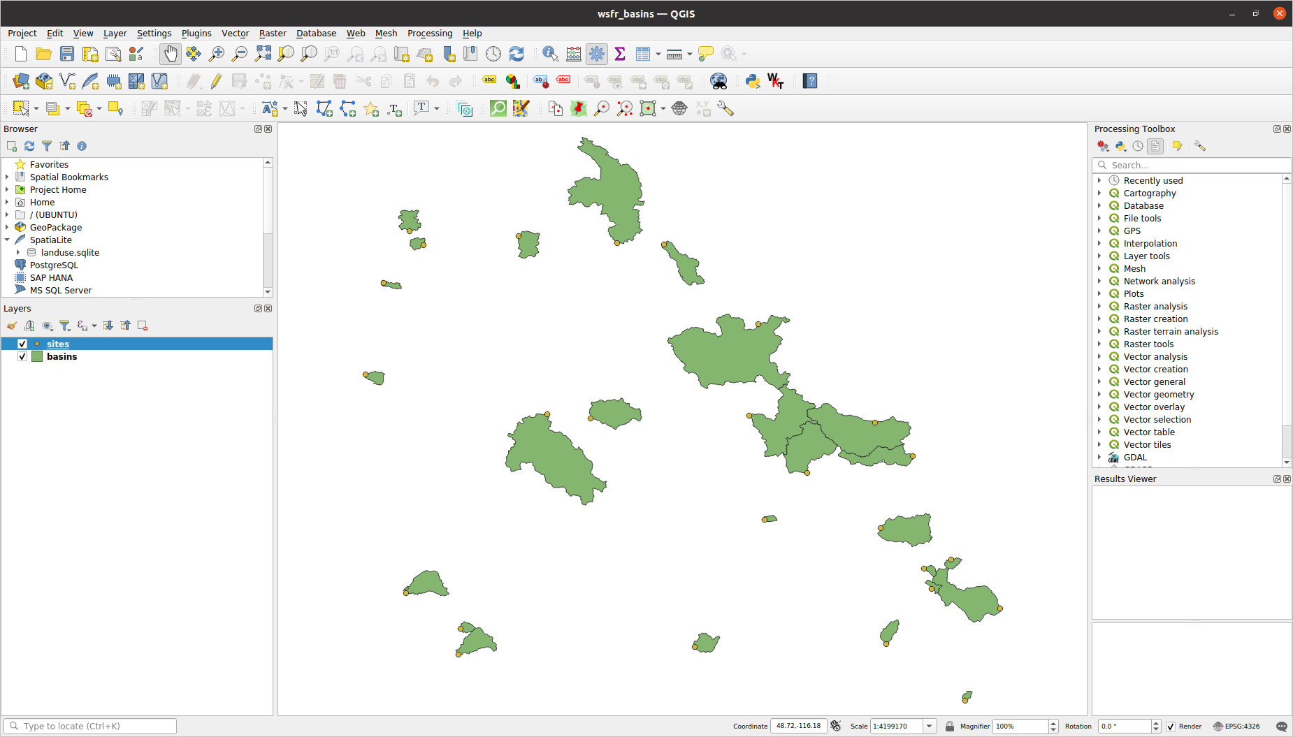
Adding state and provice boundaries
Add a new vector layer (using Data Source Manager or Layer | Add Layer | Add Vector Layer …). Set the option to Directory instead of File and set the Source Type to OpenFileGDB. Browse to the cb_2022_us_all_20m.gdb folder, select it. Click Add button. You’ll see a list of all the available layers. We just want the state boundary layer. After moving the added layer to the bottom of the map, we have something that looks like this. We’ll change the styling later.
Image('./images/add_state_boundaries.png')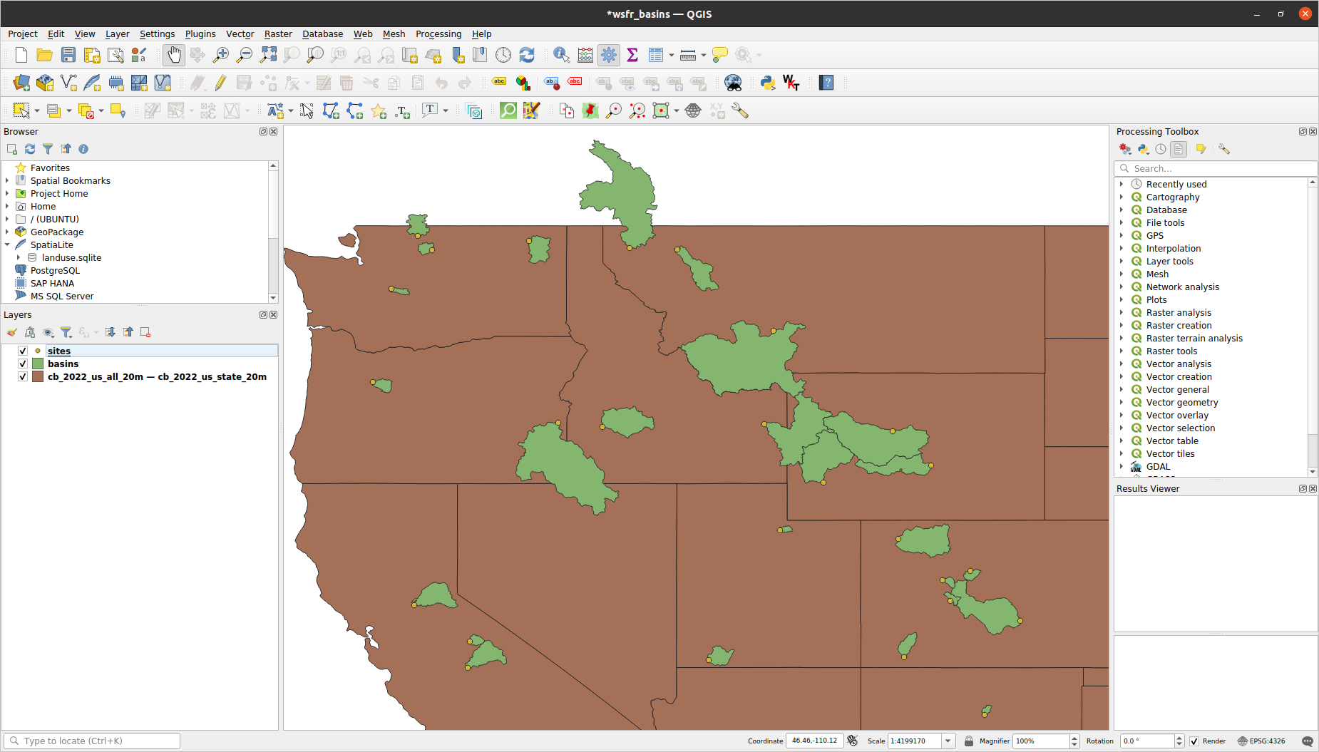
For the Canadian province borders, just add another vector layer but browse to the lpr_000b16a_e.shp shapefile that was part of the downloaded zip file.
Then change the styling of these two layers as you see fit. I gave them no fill and different colored borders.
Adding DEM layer
Add a new raster layer based on the na_con_3s.tif GeoTIFF file downloaded earlier. By default it will load as a singleband gray scale item. I changed this to a singleband pseudocolor and chose a color gradient using earth tones.
Image('./images/add_DEM.png')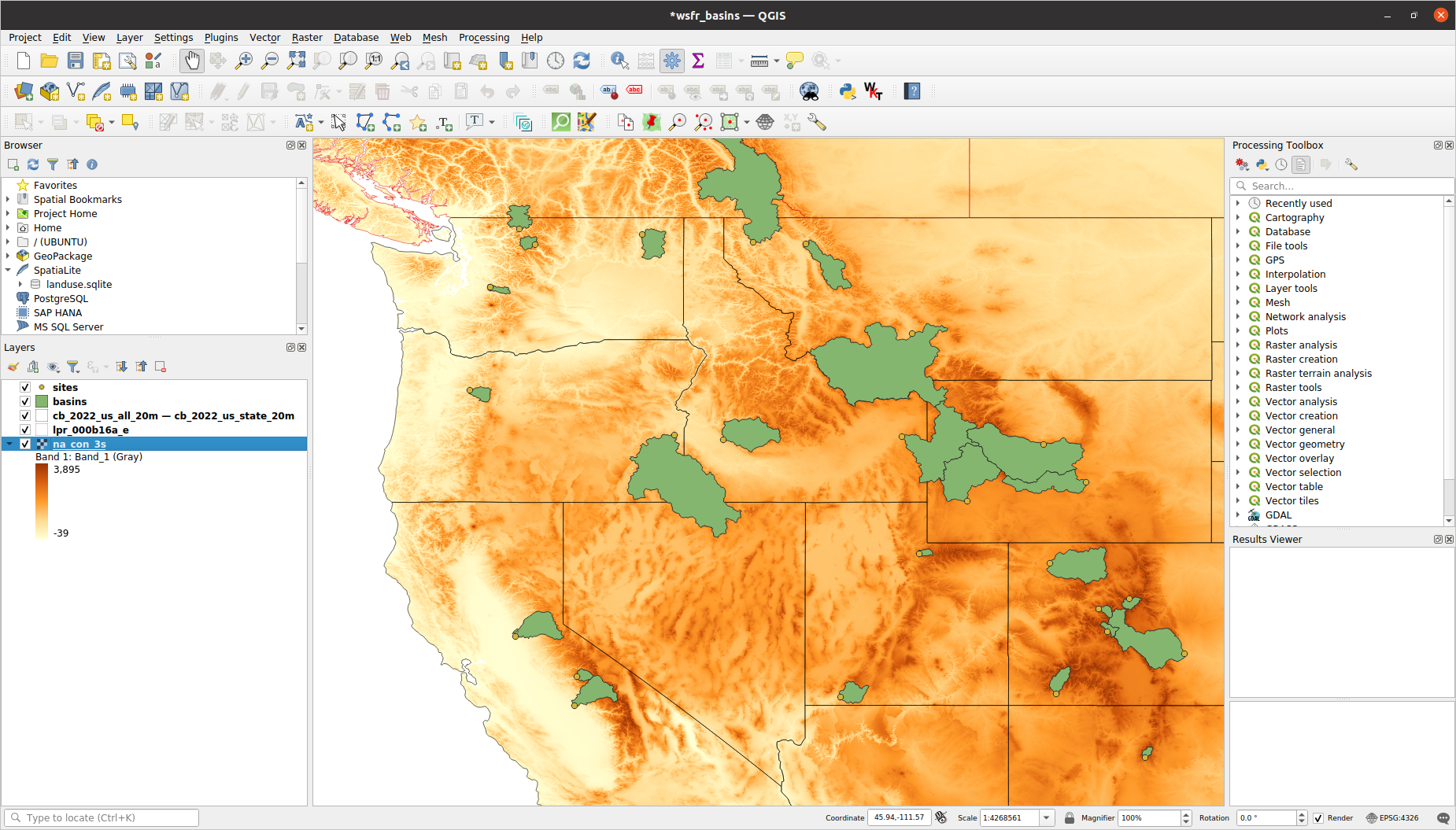
Adding rivers (vector)
Like the state boundaries, the river data is in a geodatabase folder. Be careful as when you uncompress the zip file, HydroRIVERS_v10_na.gdb.zip, you end up with a folder, HydroRIVERS_v10_na.gdb that is NOT a geodatabase. The actual geodatabase folder is inside this folder and is named HydroRIVERS_v10_na.gdb. This layer may take a bit to load as there are a lot of rivers.
I decided to filter this layer to include only rivers whose ORD_FLOW value was less than or equal to 6. You can right click on the layer and select Filter and then build the expression ORD_FLOW <= 6 or whatever you want.
From the HydroRIVERS technical documentation, the ORD_FLOW attribute is defined as:
Indicator of river order using river flow to distinguish logarithmic size classes: order 1 represents river reaches with a long-term average discharge ≥ 100,000 m 3 /s; order 2 represents river reaches with a long-term average discharge ≥ 10,000 m 3 /s and < 100,000 m 3 /s; … order 9 represents river reaches with a long-term average discharge ≥ 0.001 m 3 /s and < 0.01 m 3 /s; and order 10 represents river reaches with a long-term average discharge < 0.001 m 3 /s (i.e., 0 in the provided data due to rounding to 3 digits).
Image('./images/add_rivers.png')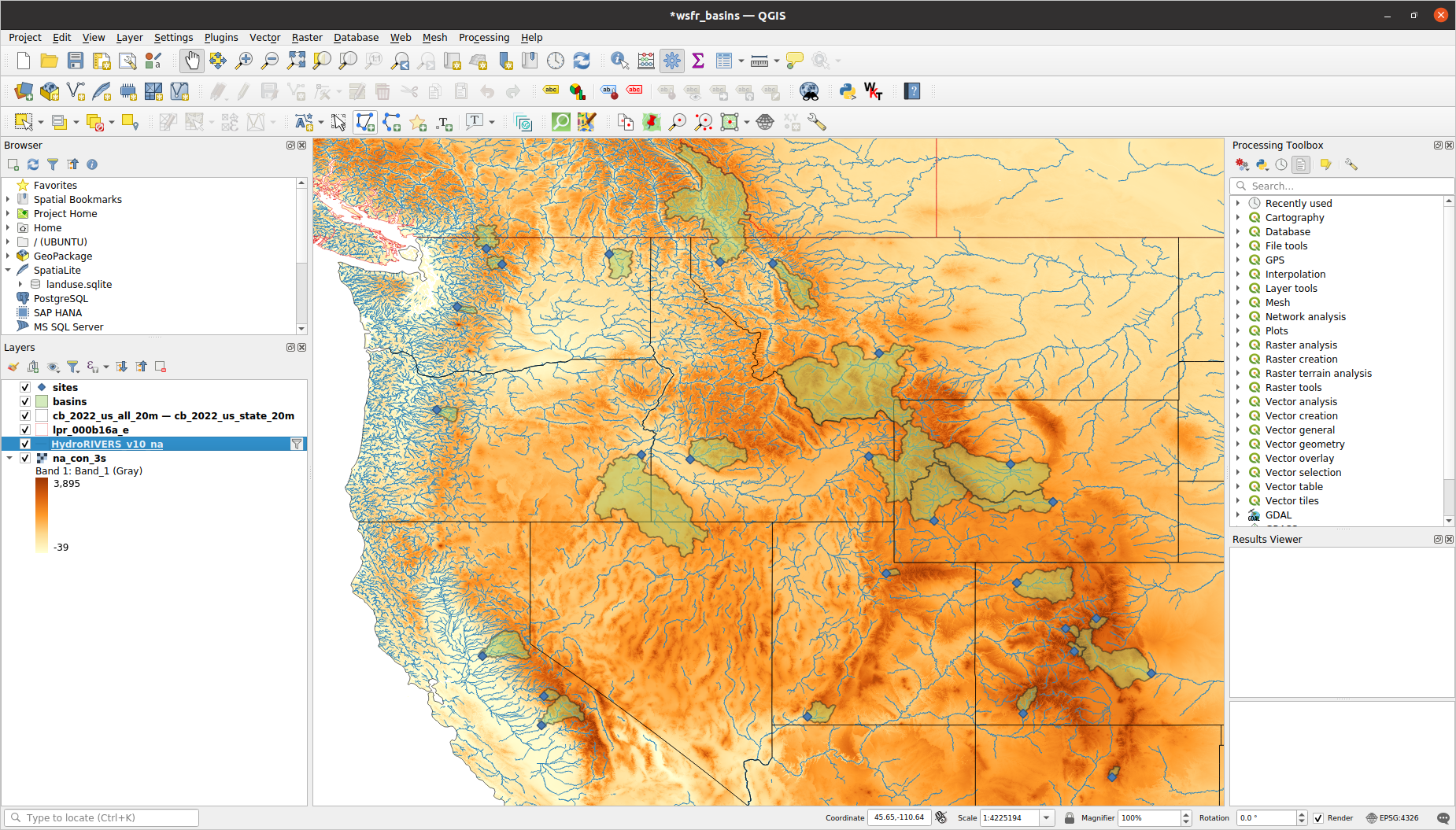
Styling changes, title and legend
I experimented with the colors and styles for the sites and basins layer until I found something I liked.
In order to add things like titles, legends, scale bar or other annotations, you need to create a new Print Layout from the main Project menu. See this QGIS documentation page for all the details.
This seemed like a good stopping point and our map looks like the first version shown in this notebook.
Now our challenge is to duplicate this map using Python and R.
Glossing over some important issues
When using QGIS, sometimes we can get a false sense of security regarding our understanding of fundamental, and often complex, issues. In particular, the above figure shows a 2D map on a screen. The world is 3D and roughly shaped like an ellipsoid. So, how exactly were the different datasets projected onto a 2D surface? What coordinate reference systems (CRS) are used in the various vector and raster datasets used? Did QGIS automatically convert all of the data to use a common CRS? In the next post, when we try to recreate the above map with Python, we’ll be forced to confront these issues, and many more. For example, here’s another version of the map above which uses what is known as the Albers Equal-Area projection. We’ll wade into the thicket that is CRSs and projections in the next post.
Image('./images/WaterSupplyForecastRodeo_Albers.png')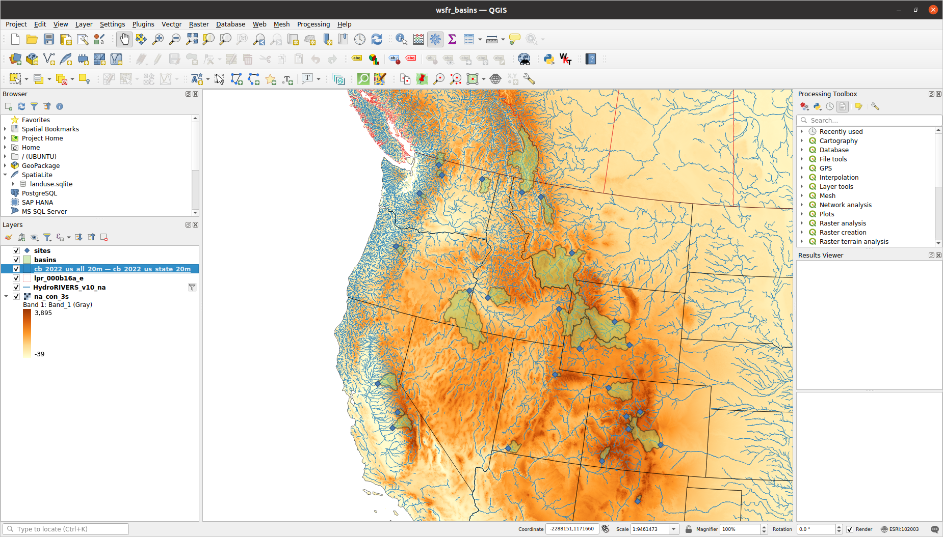
Reuse
Citation
BibTeX citation:
@online{isken2024,
  author = {Isken, Mark},
  title = {A Vector-Raster River Map, Three Ways - {Part} 1: {QGIS}},
  date = {2024-01-15},
  url = {https://bitsofanalytics.org/posts/river_map_qgis/},
  langid = {en}
}
For attribution, please cite this work as:
Isken, Mark. 2024. “A Vector-Raster River Map, Three Ways - Part
1: QGIS.” January 15. https://bitsofanalytics.org/posts/river_map_qgis/.