# Need to do some date math and need to work with file paths
from datetime import timedelta
from pathlib import PathAlgal bloom detection extended tutorial - Part 1: geospatial libraries
Making sense of Python geospatial libraries
geonewb
geospatial
python
conda
This is part of the geonewb series of posts.
I’m working through the Getting Started Tutorial that’s part of the Detecting harmful algal bloom challenge run by the Driven Data folks. Since I’ve worked just a bit with geographic and even less with image data, I’m using this challenge as a vehicle for quickly learning more about these topics.
It’s a terrific tutorial and as I was working through it I would branch off to learn more about some of the underlying concepts and technologies. This led to a mess of Jupyter notebooks and now I’m trying to bring all of that together into a somewhat extended version of the original tutorial. I’m also going to break this up into a few parts to keep the notebook sizes reasonable. In this first part we’ll focus on the following:
- an overview of the algae bloom detection challenge,
- getting a high level understanding of the myriad of geospatial Python packages we’ll be using as well as of Microsoft’s Planetary Computer
- creating a Conda virtual environment with the necessary geospatial packages.
- exploring the project data from DrivenData (metadata and training labels)
In Part 2 (and maybe 3 depending on length), we’ll cover:
- acquiring satellite image data (both Sentinel-2 and Landsat) from Microsoft’s Planetary Computer,
- build a basic understanding of the structure and data content of these satellite created images,
- basic viewing and manipulation of satellite imagery.
In subsequent parts we’ll tackle the feature engineering and predictive modeling sections of the original tutorial.
When I quote directly from the original tutorial or from other online documentation, I’ll format it as a block quote. For example, from the main project page:
Inland water bodies like lakes and reservoirs provide critical drinking water and recreation for communities, and habitats for marine life. A significant challenge that water quality managers face is the formation of harmful algal blooms (HABs) such as cyanobacteria. HABs produce toxins that are poisonous to humans and their pets, and threaten marine ecosystems by blocking sunlight and oxygen. Manual water sampling, or “in situ” sampling, is generally used to monitor cyanobacteria in inland water bodies. In situ sampling is accurate, but time intensive and difficult to perform continuously.
Your goal in this challenge is to use satellite imagery to detect and classify the severity of cyanobacteria blooms in small, inland water bodies like reservoirs. Ultimately, better awareness of algal blooms helps keep both the human and marine life that relies on these water bodies safe and healthy.
I highly recommend having the original tutorial open as you read or work through this notebook.
Python (and other) libraries for geospatial analysis
This tutorial (and geospatial analysis, in general) uses a whole bunch of libraries, each with many dependencies. Just trying to wrap your head around the main geospatial libraries and their role, is non-trivial. Then, getting them all installed into one or more conda virtual environments is also non-trivial. For example, here is a list of all of the import statements from the original tutorial (blank lines indicating a different Jupyter code cell). Actually, these are only the imports related to the sections of the tutorial before the machine learning modeling.
import cv2
from datetime import timedelta
import matplotlib.pyplot as plt
import numpy as np
import odc.stac
import pandas as pd
from pathlib import Path

import geopandas as gpd
from shapely.geometry import Point

import planetary_computer as pc
from pystac_client import Client

import geopy.distance as distance

import rioxarray
While some of these are familiar to anyone doing data science work in Python (matplotlib, numpy, pandas, datetime), there are a number of geospatial specific libraries. I started by exploring the documentation for and playing around with each of these just enough to figure out their major role in geospatial analysis. Many of these packages have important geospatial related dependencies and I’ll describe them as we run into them. After getting a high level look at these, we will try to get them installed within a conda virtual environment.
odc-stac - load STAC items into xarray DataSet
A bunch to unpack here. STAC stands for SpatioTemporal Asset Catalogs. Microsoft’s Planetary Computer API builds on STAC.
The STAC specification is a common language to describe geospatial information, so it can more easily be worked with, indexed, and discovered.
What about xarray?
xarray - labelled multidimension arrays
Xarray builds on top of NumPy N-d arrays and adds ability to create and work with labels for the dimensions.
Xarray makes working with labelled multi-dimensional arrays in Python simple, efficient, and fun!
The two main data structures are DataArray (a N-d generalization of a pandas.Series) and DataSet (an N-d generalization of a pandas.DataFrame). The Overview: Why xarray? page has a nice level of detail on the case for xarray and its link to geospatial analysis.
Open Data Cube - An Open Source Geospatial Data Management and Analysis Platform
While digging into odc-stac, it became clear that it was part of a much bigger project called Open Data Cube. The ODC project was initiated in Australia. From the main web site:
The Open Data Cube (ODC) is an Open Source Geospatial Data Management and Analysis Software project that helps you harness the power of Satellite data. At its core, the ODC is a set of Python libraries and PostgreSQL database that helps you work with geospatial raster data. See our GitHub repository here>>.
The ODC seeks to increase the value and impact of global Earth observation satellite data by providing an open and freely accessible exploitation architecture. The ODC project seeks to foster a community to develop, sustain, and grow the technology and the breadth and depth of its applications for societal benefit.
One key feature seems to be the ability to work with images over time in order to visualize the dynamics of landscape change. These time based stacks of images form the “cube”. Like the Planetary Computer and Google Earth Engine, ODC provides not just catalogued data but also a compute environment and apps for exploring data. It, again like the Planetary Computer, is based on free and open source software and is visibly committed to this for the long term.
Some key tools that are part of the ODC ecosystem are odc-stac and odc-geo. The former provides an easy way to load STAC items into xarray data structures and the latter provides:
This library combines geometry shape classes from shapely with CRS from pyproj to provide projection aware
Geometry
It seems as if these libraries were part of the ODC core but have been extracted as utilities to facilitate wider use without requiring installation of the full ODC package.
What is unclear to me is the status of the ODC project. The Latest News section’s most recent item is about its 2021 conference. There is recent activity in the opendatacube-core repo. A sandbox is available but I haven’t had time to try it out.
GeoPandas - add geospatial functionality to pandas
The basic idea is to combine the capabilites of pandas with the shapely library to allow you to work with geospatial data in a pandas-like way.
GeoPandas is an open source project to make working with geospatial data in python easier. GeoPandas extends the datatypes used by pandas to allow spatial operations on geometric types. Geometric operations are performed by shapelyhttps://shapely.readthedocs.io/en/stable/index.html. GeoPandas further depends on fiona for file access and matplotlib for plotting.
shapely - manipulation and analysis of geometric objects in the Cartesian plane
Shapely makes it easy to work with points, curves, and surfaces with Python. Shapely objects will end up as datatypes in GeoPandas dataframes (a GeoDataFrame).
fiona - Pythonic reading and writing of geospatial data
Fiona reads and writes geographic data files and thereby helps Python programmers integrate geographic information systems with other computer systems. Fiona contains extension modules that link the Geospatial Data Abstraction Library (GDAL).
So, Fiona reads and writes geographic data files in a Pythonic way using GDAL to do the heavy lifting.
So we finally get to meet the venerable GDAL library.
GDAL - the Geospatial Data Abstraction Library
GDAL is an indispensable part of computational geospatial work. What is it?
- a translator library for raster and vector geospatial data formats (a few hundred) written in C, C++ and Python,
- an open source package (MIT License) released by The Open Source Geospatial Foundation (OSGeo),
- in addition to being used as a callable library, it includes a set of command line tools,
- is used as a core resource in countless GIS and geospatial analysis tools (e.g., free and open-source packages such as QGIS and GRASS; even ESRI appears to use GDAL to deal with custom raster formats).
Another related library, OGR, is part of the GDAL source code and focuses on “simple features vector data”. This GDAL FAQ page gives more detail on the GDAL/OGR relationship. When people say GDAL, it includes OGR. Speaking of saying, both “gee-doll” and “goo-dle” are used.
GDAL/OGR also relies on the PROJ library for projections and transformations.
Given the importance of GDAL and its use by so many geospatial software packages, it is somewhat surprising that for many years it was maintained by a single person. Check out this Mapscaping podcast on GDAL for a fascinating telling of the GDAL story.
As we’ll see, we usually don’t have to install GDAL as it will get installed when we install higher level packages such as GeoPandas.
PROJ - transform geospatial coordinates between different coordinate reference systems
If you are going to work with geospatial data, you are going to have to learn about coordinate reference systems (CRS) and map projections. The world isn’t flat and it’s not a perfect sphere. However, most maps are flat. Projections are a way of translating our non-flat earth to a flat representation for mapping. The CRS is a specific type of “grid system” so that numeric X-Y coordinates can be associated with any point on the map.
A great source of Python flavored introductory material on things like CRS and projections and general GIS concepts is the open source book - PyGIS: Python Open Source Spatial Programming & Remote Sensing. The QGIS documentation also has a good overview of these topics. Then you’ll want to learn about the World Geodesic System (WGS) and things like EPSG codes. For example, EPSG:4326 - WGS 84 is the latitude/longitude coordinate system based on the Earth’s center of mass, used by GPS and in many mapping applications.
The PROJ library does the heavy lifting of translating between different CRS and projections. Much like GDAL, it is
- open source,
- used both as a library and command line tool,
- foundational software to geospatial analysis,
- now maintained by OSGeo.
While the underlying library is C/C++, you can use PROJ from Python via the pyproj package. Like GDAL, pyproj will get installed when we install a higher level package such as GeoPandas. However, there are several different ways to install PROJ and early on I seem to have found one that resulted in multiple (and conflicting) PROJ installations on my Linux machine. Eventually I fixed it - more on this later.
planetary_computer - data, API, compute, ecosystem for earth observation
Microsoft’s, pretty new, Planetary Computer is quite an amazing project. It has several major components:
- Data Catalog - It is a ginormous repository of well cataloged data all about Earth’s various systems and includes a web based interface that allows users to find relevant data - for free.
- API - It has an API that leverages open source tools to make it easy to do data searches by time and location. Focuses on Python.
- Hub - A managed compute environment for doing cloud based geospatial analysis at scale. For this part you need to apply for access.
- Applications - an ecosystem of people doing meaningful work with the Planetary Computer.
There’s a really good Mapscaping podcast featuring two of the main developers of the Planetary Computer - see https://mapscaping.com/podcast/the-planetary-computer/. The Mapscaping.com site is a great place to learn about geospatial analysis through its terrific podcasts. For example, when I started going through the algae bloom tutorial, it mentioned two primary sources for obtaining free satellite imagery data - Microsoft’s Planetary Computer and the Google Earth Engine. Which should I use? Did a bunch of reading, where I also learned about this thing called the Sentinel Hub, but really benefited from Daniel O’Donohue’s (the podcaster behind Mapscaping.com) series of podcasts:
- The Planetary Computer - https://mapscaping.com/podcast/the-planetary-computer/
- Introducing Google Earth Engine - https://mapscaping.com/podcast/introducing-google-earth-engine/
- Sentinel Hub - https://mapscaping.com/podcast/sentinel-hub/
We’ll mostly be using the Planetary Computer to search for and acquire satellite image data from the Sentinel-2 and Landsat catalogs. We can use pystac-client to do this freely and without any authentication. As mentioned above, authentication is required to use the Hub computing cluster.
PySTAC - A Python library for working with STACs
The PySTAC package provides a Python based way of creating and working with the fundamental building blocks of STACs - catalogs, collections, and items. STAC itself is a specification. PySTAC provides tools to enable STAC compliant development. There are a few related projects (taken directly from the PySTAC docs):
- pystac-client: A Python client for working with STAC Catalogs and APIs.
- stactools: A command line tool and library for working with STAC.
- sat-stac: A Python 3 library for reading and working with existing Spatio-Temporal Asset Catalogs (STAC). Much of PySTAC builds on the code and concepts of sat-stac.
pystac-client - A Python client for working with STAC Catalogs and APIs
Microsoft’s Planetary Computer is heavily based on the STAC specification. The pystac-client package provides the tools we need to interact with the Planetary Computer API. In particular, it provides search related functionality.
geopy - Python client for several popular geocoding web services
The geopy library makes it easier to interact with different geocoding services (e.g. Google Maps) by avoiding having to work with their individual APIs.
While geopy’s primary role is as a way to use Python with web-based geocoding services, it has some functions that are useful for more basic geospatial analysis needs. In particular, the geopy library includes a geodesic distance function that we can use to find a bounding box of a specific size. A bounding box is a rectangular area defined by two latitude values and two longitude values - it’s often abbreviated as a bbox.
The geodesic distance is the shortest distance on the surface of an ellipsoidal model of the earth. The default algorithm uses the method is given by Karney (2013) (geodesic); this is accurate to round-off and always converges.
The default elipsoid is WGS-84, but this can be changed.
rioxarray - read raster data into xarray objects
The rioxarray package extends the xarray package to facilitate reading raster data into xarray objects. The actual reading of the raster file is done using another Python package known as rasterio. From the rasterio docs:
Geographic information systems use GeoTIFF and other formats to organize and store gridded raster datasets such as satellite imagery and terrain models. Rasterio reads and writes these formats and provides a Python API based on Numpy N-dimensional arrays and GeoJSON.
Before rasterio came along, we had use Python bindings to GDAL.
Before Rasterio there was one Python option for accessing the many different kind of raster data files used in the GIS field: the Python bindings distributed with the Geospatial Data Abstraction Library, GDAL. These bindings extend Python, but provide little abstraction for GDAL’s C API. This means that Python programs using them tend to read and run like C programs.
This GIS Stack Exchange post shows a simple example of using rioxarray to read a raster file and get at the data values in the underlying xarray DataArray.
And, this GIS Stack Exchange post xplains how rioxarray combines rasterio with xarray to make it easier to work with raster data in Python. It’s similar to how GeoPandas combines functionality from pandas, shapely and fiona.
GIS Stack Exchange is like StackOverflow for geospatial questions. Very helpful.
cv2 - computer vision
The cv2 module is actually part of the opencv library which supplies Python bindings for the underlying C++ based OpenCV library. For historical reasons, they’ve stayed with import cv2. This library contains hundreds of computer vision related functions and tools.
Creating a Conda virtual environment for this geospatial tutorial
Welp, that’s a lot of packages. My first inclination was to create a conda environment YAML file with everything in there and just let it rip. That turned out like you might think - hung forever at the “solving environment” stage and needed to be interupted. Then I tried creating a minimal conda environment and installing the geospatial packages as needed as I worked through the tutorial. I always tried to use conda to do the install, but had to resort to pip for a few things. That also turned out like you might think - things ran for a while but eventually I must have created a dependency conflict and the environment was gorked. Time to be more strategic. I noticed that GeoPandas has a ton of dependencies and figured I’d start by just installing it first and seeing which other packages I needed ended up being installed as a dependency.
Here’s the conda gp_39.yml env file for a minimal GeoPandas install.
# Minimal install of GeoPandas
name: gp_39
channels:
  - defaults
  - conda-forge
dependencies:
  - python=3.9
  - geopandas
# Make environment discoverable by JupyterLab
  - ipykernel
# Environment level pip for eventual pip installs
  - pip
I created the enironment:
conda env create -f gp_39.ymland then listed the installed packages after it was done:
conda activate gp_39
conda list
Here are the relevant geospatial (and data science) packages that got installed when the gp_39 conda environment was created.
fiona                     1.8.22           py39h417a72b_0

gdal                      3.0.2            py39h40f10ac_6
geopandas                 0.9.0                      py_1
geopandas-base            0.9.0                      py_1
geos                      3.8.0                he6710b0_0
geotiff                   1.7.0                hd69d5b1_0

numpy                     1.23.5           py39h14f4228_0
numpy-base                1.23.5           py39h31eccc5_0

pandas                    1.5.2            py39h417a72b_0

pillow                    9.3.0            py39hace64e9_1
pip                       22.3.1           py39h06a4308_0

proj                      6.2.1                h05a3930_0

pyproj                    2.6.1.post1      py39hb3025e9_1

scikit-learn              1.2.0            py39h6a678d5_0
scipy                     1.9.3            py39h14f4228_0

shapely                   1.8.4            py39h81ba7c5_0
Some of things that did NOT get installed, but that we’ll need (maybe) are:
- xarray
- rioxarray
- planetary_computer
- pystac-client
- geopy
- opencv
- odc-stac
Mixing conda installs with pip installs is a tricky business and it’s really important to install everything you can via conda before mixing in pip installs. Of the packages above, the following seem to suggest that a conda install is possible or even suggested:
- rioxarray
- xarray (this will get installed by rioxarray)
- geopy
- planetary-computer
- pystac-client
Next I installed planetary-computer from the conda-forge channel.
conda install -c conda-forge planetary-computerInstalling planetary-computer also installed pystac-client.
Next was geopy and then rioxarray. I looked at the dependencies for rioxarray on conda-forge and see the following:
- python >=3.8
- rasterio >=1.1.1
- scipy
- xarray >=0.17
- pyproj >=2.2
- packaging
The pyproj dependency is already met. The main conda channel has version 1.2.10 of rasterio and version 0.20.1 of rasterio - so we should be good there.
conda install -c conda-forge geopy
conda install -c conda-forge rioxarray
Both installed with no issues. I think that my early PROJ conflict was due to improperly installing rioxarray.
At this point, the only two packages that are not part of our virtual environment are opencv and odc-stac. In reading through the tutorial, these were only used for processing Landsat data. In particular, opencv was used to normalize Landsat imagery values to a 0-255 scale and odc-stac seemed like it was doing a job that pystac-client could do. Given the issues I had with installing these two packages, I decided to just not install them and either find another or implement my own normalization function - we’ll see this in a later part of this series of posts.
UPDATE 2023-01-29 Realized my odc-stac install problems were due to my own ill advised mixing of pip and conda installs. Did the following and now odc-stac installed and working just fine.
conda install -c conda-forge odc-stacWith our conda environment in place, we are ready to explore the project data.
Project data from DrivenData
The three main datafiles are available from https://www.drivendata.org/competitions/143/tick-tick-bloom/data/.
- Metadata - Metadata for both train and test set
- Train labels - Cyanobacteria labels for the train set
- Submission format - Format for submissions, with a placeholder for severity
Labels in this competition are based on “in situ” samples that were collected manually and then analyzed for cyanobacteria density. Each measurement is a unique combination of date and location (latitude and longitude).
There are three data files available in the download. Acquisition of the actual image data that is needed to create modeling features will be the primary focus of this part of the tutorial.
.
├── metadata.csv
├── submission_format.csv
└── train_labels.csv
I just followed the data folder structure used in the tutorial.
Library imports and data directory setup
We’ll load a few libraries up front. For the rest, we will load as needed.
# Big 3 - come on, of course you'll need these
import matplotlib.pyplot as plt
import numpy as np
import pandas as pd%matplotlib inlineDATA_DIR = Path.cwd().resolve() / "data/final/public"
assert DATA_DIR.exists()Let’s explore each of the data files.
Explore the metadata (metadata.csv)
The metadata tells us where each unique sample was taken and whether it is part of the train or test data.
metadata = pd.read_csv(DATA_DIR / "metadata.csv", parse_dates=['date'])
metadata.head()| uid | latitude | longitude | date | split | |
|---|---|---|---|---|---|
| 0 | aabm | 39.080319 | -86.430867 | 2018-05-14 | train |
| 1 | aabn | 36.559700 | -121.510000 | 2016-08-31 | test |
| 2 | aacd | 35.875083 | -78.878434 | 2020-11-19 | train |
| 3 | aaee | 35.487000 | -79.062133 | 2016-08-24 | train |
| 4 | aaff | 38.049471 | -99.827001 | 2019-07-23 | train |
metadata.info()<class 'pandas.core.frame.DataFrame'>
RangeIndex: 23570 entries, 0 to 23569
Data columns (total 5 columns):
# Column Non-Null Count Dtype
--- ------ -------------- -----
0 uid 23570 non-null object
1 latitude 23570 non-null float64
2 longitude 23570 non-null float64
3 date 23570 non-null datetime64[ns]
4 split 23570 non-null object
dtypes: datetime64[ns](1), float64(2), object(2)
memory usage: 920.8+ KBThe field defs are:
uid (str): unique ID for each row. Each row is a unique combination of date and location (latitude and longitude).date (pd.datetime): date when the sample was collected, in the format YYYY-MM-DDlatitude (float): latitude of the location where the sample was collectedlongitude (float): longitude of the location where the sample was collectedregion (str): region of the US. This will be used in scoring to calculate region-specific RMSEs. Final score will be the average across the four US regions.split (str): indicates whether the row is part of the train set or the test set. Metadata is provided for all points in the train and test sets.
Let’s look at the size of the training and test data.
metadata.groupby(['split']).count()| uid | latitude | longitude | date | |
|---|---|---|---|---|
| split | ||||
| test | 6510 | 6510 | 6510 | 6510 |
| train | 17060 | 17060 | 17060 | 17060 |
metadata.split.value_counts(dropna=False)train 17060
test 6510
Name: split, dtype: int64The geographic points in the train and test sets are distinct. This means that none of the test set points are also in the train set, so your model’s performance will be measured on unseen locations.
The main feature data for this competition is satellite imagery from Sentinel-2 and Landsat. Participants will access all feature data through external, publicly available APIs. Relevant imagery can be identified using the location and date of each sample from the metadata.
# Confirm all uid are unique
metadata['uid'].nunique()23570metadata.groupby(['split'])['uid'].nunique()split
test 6510
train 17060
Name: uid, dtype: int64Distribution of samples by location
Ok, time to start learning more about location data. Here is where GeoPandas and shapely will come in handy.
import geopandas as gpd
from shapely.geometry import Point
First we load a base map upon which to plot the points.
# load the default geopandas base map file to plot points on
world = gpd.read_file(gpd.datasets.get_path("naturalearth_lowres"))world.plot();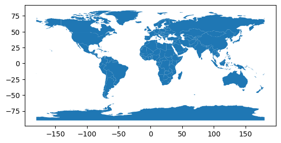
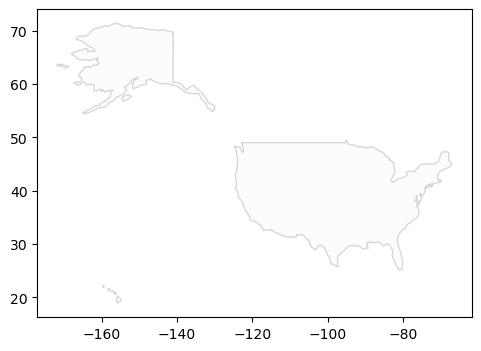
Now, let’s just plot the USA.
fig, ax = plt.subplots(figsize=(9, 4))

base = world[world.name == "United States of America"].plot(
    edgecolor="gray", color="ghostwhite", figsize=(9, 4), alpha=0.3, ax=ax
)
Before going any further, let’s explore the underlying GeoDataFrame.
world.info()<class 'geopandas.geodataframe.GeoDataFrame'>
RangeIndex: 177 entries, 0 to 176
Data columns (total 6 columns):
# Column Non-Null Count Dtype
--- ------ -------------- -----
0 pop_est 177 non-null int64
1 continent 177 non-null object
2 name 177 non-null object
3 iso_a3 177 non-null object
4 gdp_md_est 177 non-null float64
5 geometry 177 non-null geometry
dtypes: float64(1), geometry(1), int64(1), object(3)
memory usage: 8.4+ KBworld.head(25)| pop_est | continent | name | iso_a3 | gdp_md_est | geometry | |
|---|---|---|---|---|---|---|
| 0 | 920938 | Oceania | Fiji | FJI | 8374.0 | MULTIPOLYGON (((180.00000 -16.06713, 180.00000... |
| 1 | 53950935 | Africa | Tanzania | TZA | 150600.0 | POLYGON ((33.90371 -0.95000, 34.07262 -1.05982... |
| 2 | 603253 | Africa | W. Sahara | ESH | 906.5 | POLYGON ((-8.66559 27.65643, -8.66512 27.58948... |
| 3 | 35623680 | North America | Canada | CAN | 1674000.0 | MULTIPOLYGON (((-122.84000 49.00000, -122.9742... |
| 4 | 326625791 | North America | United States of America | USA | 18560000.0 | MULTIPOLYGON (((-122.84000 49.00000, -120.0000... |
| 5 | 18556698 | Asia | Kazakhstan | KAZ | 460700.0 | POLYGON ((87.35997 49.21498, 86.59878 48.54918... |
| 6 | 29748859 | Asia | Uzbekistan | UZB | 202300.0 | POLYGON ((55.96819 41.30864, 55.92892 44.99586... |
| 7 | 6909701 | Oceania | Papua New Guinea | PNG | 28020.0 | MULTIPOLYGON (((141.00021 -2.60015, 142.73525 ... |
| 8 | 260580739 | Asia | Indonesia | IDN | 3028000.0 | MULTIPOLYGON (((141.00021 -2.60015, 141.01706 ... |
| 9 | 44293293 | South America | Argentina | ARG | 879400.0 | MULTIPOLYGON (((-68.63401 -52.63637, -68.25000... |
| 10 | 17789267 | South America | Chile | CHL | 436100.0 | MULTIPOLYGON (((-68.63401 -52.63637, -68.63335... |
| 11 | 83301151 | Africa | Dem. Rep. Congo | COD | 66010.0 | POLYGON ((29.34000 -4.49998, 29.51999 -5.41998... |
| 12 | 7531386 | Africa | Somalia | SOM | 4719.0 | POLYGON ((41.58513 -1.68325, 40.99300 -0.85829... |
| 13 | 47615739 | Africa | Kenya | KEN | 152700.0 | POLYGON ((39.20222 -4.67677, 37.76690 -3.67712... |
| 14 | 37345935 | Africa | Sudan | SDN | 176300.0 | POLYGON ((24.56737 8.22919, 23.80581 8.66632, ... |
| 15 | 12075985 | Africa | Chad | TCD | 30590.0 | POLYGON ((23.83766 19.58047, 23.88689 15.61084... |
| 16 | 10646714 | North America | Haiti | HTI | 19340.0 | POLYGON ((-71.71236 19.71446, -71.62487 19.169... |
| 17 | 10734247 | North America | Dominican Rep. | DOM | 161900.0 | POLYGON ((-71.70830 18.04500, -71.68774 18.316... |
| 18 | 142257519 | Europe | Russia | RUS | 3745000.0 | MULTIPOLYGON (((178.72530 71.09880, 180.00000 ... |
| 19 | 329988 | North America | Bahamas | BHS | 9066.0 | MULTIPOLYGON (((-78.98000 26.79000, -78.51000 ... |
| 20 | 2931 | South America | Falkland Is. | FLK | 281.8 | POLYGON ((-61.20000 -51.85000, -60.00000 -51.2... |
| 21 | 5320045 | Europe | Norway | -99 | 364700.0 | MULTIPOLYGON (((15.14282 79.67431, 15.52255 80... |
| 22 | 57713 | North America | Greenland | GRL | 2173.0 | POLYGON ((-46.76379 82.62796, -43.40644 83.225... |
| 23 | 140 | Seven seas (open ocean) | Fr. S. Antarctic Lands | ATF | 16.0 | POLYGON ((68.93500 -48.62500, 69.58000 -48.940... |
| 24 | 1291358 | Asia | Timor-Leste | TLS | 4975.0 | POLYGON ((124.96868 -8.89279, 125.08625 -8.656... |
The world object is a pandas DataFrame with one of the columns being a GeoSeries having a geometry data type. You can have multiple such columns but only one geometry is active at a time. Each row is a country.
world[world['iso_a3'] == 'USA']| pop_est | continent | name | iso_a3 | gdp_md_est | geometry | |
|---|---|---|---|---|---|---|
| 4 | 326625791 | North America | United States of America | USA | 18560000.0 | MULTIPOLYGON (((-122.84000 49.00000, -120.0000... |
The MULTIPOLYGON object is from the shapely library.
world[world['iso_a3'] == 'USA']['geometry']4 MULTIPOLYGON (((-122.84000 49.00000, -120.0000...
Name: geometry, dtype: geometryLet’s recreate the plot but overlay the sample points.
fig, ax = plt.subplots(figsize=(9, 4))

# map the training data
base = world[world.name == "United States of America"].plot(
    edgecolor="gray", color="ghostwhite", figsize=(9, 4), alpha=0.3, ax=ax
)
# Subset the `metadata` dataframe
train_meta = metadata[metadata["split"] == "train"]
# Create a list of `Point` (a shapely data type) objects based on the lat-long columns
geometry = [Point(xy) for xy in zip(train_meta["longitude"], train_meta["latitude"])]
# Create a new GeoDataFrame from the training data and the geometry (list of shapely Point objects) we just created
gdf = gpd.GeoDataFrame(train_meta, geometry=geometry)
# Plot the training data in blue
gdf.plot(ax=base, marker=".", markersize=3, color="blue", label="Train", alpha=0.6)

# map the test data - same steps as above, but plot in orange
test_meta = metadata[metadata["split"] == "test"]
geometry = [Point(xy) for xy in zip(test_meta["longitude"], test_meta["latitude"])]
gdf = gpd.GeoDataFrame(test_meta, geometry=geometry)
gdf.plot(ax=base, marker=".", markersize=3, color="orange", label="Test", alpha=0.6)

plt.xlabel("Longitude")
plt.ylabel("Latitude")
# Set x and y axis limits to just show the continental USA
plt.xlim([-125, -65])
plt.ylim([25, 50])
plt.legend(loc=4, markerscale=3)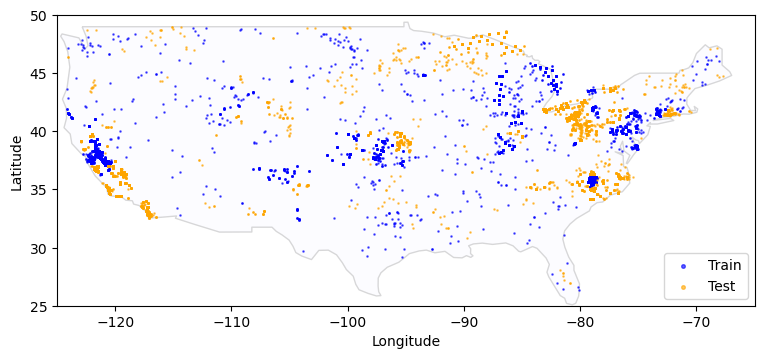
Before moving on, let’s look at the geometry list of Point data.
geometry[0:5][<shapely.geometry.point.Point at 0x7fbd961c5d60>,
<shapely.geometry.point.Point at 0x7fbd964c3d90>,
<shapely.geometry.point.Point at 0x7fbd964a9760>,
<shapely.geometry.point.Point at 0x7fbd961eb910>,
<shapely.geometry.point.Point at 0x7fbd961eb790>]first_point = geometry[0]
print(first_point)POINT (-121.51 36.5597)Points aren’t going to have too many attributes beyond their location.
print(f'A point has an area of {first_point.area}')
print(f'This point has a centroid at {first_point.centroid}')
A point has an area of 0.0
This point has a centroid at POINT (-121.51 36.5597)This was my first time using GeoPandas + matplotlib to create maps and found it pretty simple to pick up. I had used R’s ggmap package a bit and this felt kind of similar (yes, ggplot2 is amazing but R users should have little problem doing mapping in Python). I’m planning on doing some similar geonewb posts on geospatial analysis in R.
Distribution of samples over time
# Let's get min and max values for all the fields.
metadata.groupby(['split']).agg(['min', 'max'])| uid | latitude | longitude | date | |||||
|---|---|---|---|---|---|---|---|---|
| min | max | min | max | min | max | min | max | |
| split | ||||||||
| test | aabn | zzzi | 26.94453 | 48.97325 | -124.0352 | -67.69865 | 2013-01-08 | 2021-12-29 |
| train | aabm | zzyb | 26.38943 | 48.90706 | -124.1792 | -68.06507 | 2013-01-04 | 2021-12-14 |
# Another way to check just the date range using "named aggregations"
metadata.groupby("split").agg(min_date=("date", min), max_date=("date", max))| min_date | max_date | |
|---|---|---|
| split | ||
| test | 2013-01-08 | 2021-12-29 |
| train | 2013-01-04 | 2021-12-14 |
Let’s plot the number of records by year. We can use pandas crosstab to get a plottable dataframe.
recs_by_split_year = pd.crosstab(metadata.date.dt.year, metadata.split)
recs_by_split_year| split | test | train |
|---|---|---|
| date | ||
| 2013 | 521 | 1362 |
| 2014 | 602 | 1504 |
| 2015 | 527 | 2299 |
| 2016 | 625 | 2428 |
| 2017 | 1031 | 2435 |
| 2018 | 777 | 1940 |
| 2019 | 1199 | 1788 |
| 2020 | 546 | 1706 |
| 2021 | 682 | 1598 |
# Quick plot with pandas plot()
recs_by_split_year.plot(kind="bar");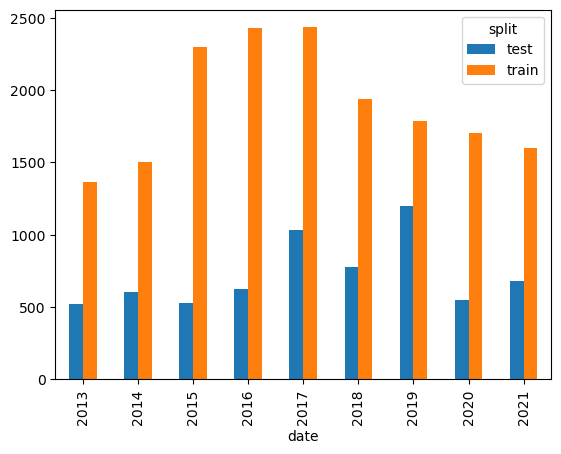
metadata.groupby([metadata.date.dt.year, metadata.date.dt.month])['uid'].count().plot(kind="line");
# what seasons are the data points from?
metadata["season"] = (
    metadata.date.dt.month.replace([12, 1, 2], "winter")
    .replace([3, 4, 5], "spring")
    .replace([6, 7, 8], "summer")
    .replace([9, 10, 11], "fall")
)
metadata.season.value_counts()
summer 10813
spring 5045
fall 4758
winter 2954
Name: season, dtype: int64Since summer is usually associated with algal blooms, it’s not surprising that it’s sampled more frequently.
Harmful algal blooms are more likely to be dangerous during the summer because more individuals are taking advantage of water bodies like lakes for recreation.
Create a separate map for each season.
# where is data from for each season?
fig, axes = plt.subplots(2, 2, figsize=(10, 5))

# Since axes is a 2x2, we'll flatten it to a vector with four elements
for season, ax in zip(metadata.season.unique(), axes.flatten()):
    base = world[world.name == "United States of America"].plot(
        edgecolor="gray", color="ghostwhite", alpha=0.3, ax=ax
    )

    sub = metadata[metadata.season == season]
    geometry = [Point(xy) for xy in zip(sub["longitude"], sub["latitude"])]
    gdf = gpd.GeoDataFrame(sub, geometry=geometry)
    gdf.plot(ax=base, marker=".", markersize=2.5)
    ax.set_xlim([-125, -66])
    ax.set_ylim([25, 50])
    ax.set_title(f"{season.capitalize()} data points")
    ax.axis("off")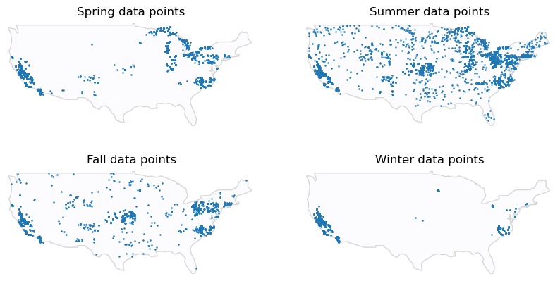
That’s a good start in exploring metadata.csv. On to the training data.
Explore the training data (train_labels.csv)
train_labels = pd.read_csv(DATA_DIR / "train_labels.csv")
train_labels.head()| uid | region | severity | density | |
|---|---|---|---|---|
| 0 | aabm | midwest | 1 | 585.0 |
| 1 | aacd | south | 1 | 290.0 |
| 2 | aaee | south | 1 | 1614.0 |
| 3 | aaff | midwest | 3 | 111825.0 |
| 4 | aafl | midwest | 4 | 2017313.0 |
train_labels.shape(17060, 4)We have one row per in situ sample. Each row is a unique combination of date and location (latitude + longitude). There are columns for:
uid (str): unique ID for each row. The uid maps each row in train_labels.csv to metadata.csvregion (str): US region in which the sample was taken. Scores are calculated separately for each of these regions, and then averaged. See the Problem Description page for details.severity (int): severity level based on the cyanobacteria density. This is what you’ll be predicting.density (float): raw measurement of total cyanobacteria density in cells per milliliter (mL)
Join the training data with the metadata so that we have access to the lat, long and date fields.
train_labels_and_metadata = train_labels.merge(
    metadata, how="left", left_on="uid", right_on="uid", validate="1:1"
)
train_labels_and_metadata| uid | region | severity | density | latitude | longitude | date | split | season | |
|---|---|---|---|---|---|---|---|---|---|
| 0 | aabm | midwest | 1 | 585.0 | 39.080319 | -86.430867 | 2018-05-14 | train | spring |
| 1 | aacd | south | 1 | 290.0 | 35.875083 | -78.878434 | 2020-11-19 | train | fall |
| 2 | aaee | south | 1 | 1614.0 | 35.487000 | -79.062133 | 2016-08-24 | train | summer |
| 3 | aaff | midwest | 3 | 111825.0 | 38.049471 | -99.827001 | 2019-07-23 | train | summer |
| 4 | aafl | midwest | 4 | 2017313.0 | 39.474744 | -86.898353 | 2021-08-23 | train | summer |
| ... | ... | ... | ... | ... | ... | ... | ... | ... | ... |
| 17055 | zzsv | south | 3 | 113125.0 | 38.707825 | -75.080867 | 2018-06-27 | train | summer |
| 17056 | zzuq | south | 3 | 175726.0 | 35.794000 | -79.015368 | 2015-08-06 | train | summer |
| 17057 | zzwo | midwest | 2 | 48510.0 | 39.792190 | -99.971050 | 2017-06-19 | train | summer |
| 17058 | zzwq | south | 1 | 1271.0 | 35.794000 | -79.012551 | 2015-03-24 | train | spring |
| 17059 | zzyb | south | 1 | 9682.0 | 35.742000 | -79.238600 | 2016-11-21 | train | fall |
17060 rows × 9 columns
severity_counts = (
    train_labels.replace(
        {
            "severity": {
                1: "1 (<20,000)",
                2: "2 (20,000-100,000)",
                3: "3 (100,000 - 1,000,000)",
                4: "4 (1,00,000 - 10,000,000)",
                5: "5 (>10,000,00)",
            }
        }
    )
    .severity.value_counts()
    .sort_index(ascending=False)
)
print(severity_counts)
plt.barh(severity_counts.index, severity_counts.values)
plt.xlabel("Number of samples")
plt.ylabel("Severity (range in cells/mL)")
plt.title("Train labels severity level counts")
5 (>10,000,00) 58
4 (1,00,000 - 10,000,000) 3547
3 (100,000 - 1,000,000) 2719
2 (20,000-100,000) 3239
1 (<20,000) 7497
Name: severity, dtype: int64Text(0.5, 1.0, 'Train labels severity level counts')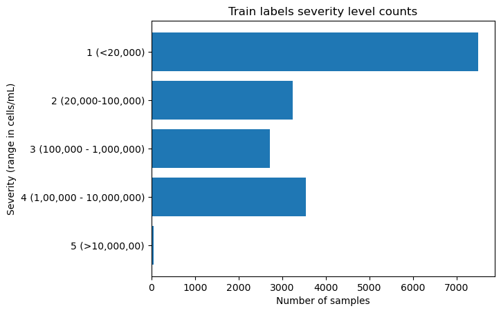
train_labels.density.describe()count 1.706000e+04
mean 1.074537e+06
std 6.836693e+06
min 0.000000e+00
25% 4.066000e+03
50% 3.270975e+04
75% 4.849192e+05
max 8.046675e+08
Name: density, dtype: float64plt.hist(train_labels.density, bins=30, range=(0.0, 1000000))(array([8570., 1394., 772., 465., 342., 244., 194., 163., 132.,
140., 101., 85., 78., 73., 77., 65., 55., 59.,
55., 49., 38., 59., 39., 33., 24., 31., 24.,
34., 28., 32.]),
array([ 0. , 33333.33333333, 66666.66666667,
100000. , 133333.33333333, 166666.66666667,
200000. , 233333.33333333, 266666.66666667,
300000. , 333333.33333333, 366666.66666667,
400000. , 433333.33333333, 466666.66666667,
500000. , 533333.33333333, 566666.66666667,
600000. , 633333.33333333, 666666.66666667,
700000. , 733333.33333333, 766666.66666667,
800000. , 833333.33333333, 866666.66666667,
900000. , 933333.33333333, 966666.66666667,
1000000. ]),
<BarContainer object of 30 artists>)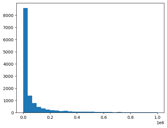
How many records have a density value of 0?
train_labels[train_labels['density'] == 0].groupby(['region'])['uid'].count()region
midwest 12
northeast 77
south 1
west 1
Name: uid, dtype: int64Explore the submission data (submission_format.csv)
submission_format = pd.read_csv(DATA_DIR / "submission_format.csv", index_col=0)
submission_format.head()| region | severity | |
|---|---|---|
| uid | ||
| aabn | west | 1 |
| aair | west | 1 |
| aajw | northeast | 1 |
| aalr | midwest | 1 |
| aalw | west | 1 |
uid (str): unique ID for each row. The uid maps each row in train_labels.csv to metadata.csvregion (str): US region in which the sample was taken. Scores are calculated separately for each of these regions, and then averaged. See the Problem Description page for details.severity (int): placeholder for severity level based on the cyanobacteria density - all values are 0. This is the column that you will replace with your own predictions to create a submission. Participants should submit predictions for severity level, NOT for the raw cell density value in cells per mL.
submission_format.shape(6510, 2)A good place to stop for part 1
We’ve got a Python conda environment for geospatial analysis and have used some of the libraries as we explored the project data files. Now we’re ready to tackle the satellite imagery data in part 2.
Reuse
Citation
BibTeX citation:
@online{isken2023,
  author = {Isken, Mark},
  title = {Algal Bloom Detection Extended Tutorial - {Part} 1:
    Geospatial Libraries},
  date = {2023-01-25},
  url = {https://bitsofanalytics.org/posts/algaebloom-part1/},
  langid = {en}
}
For attribution, please cite this work as:
Isken, Mark. 2023. “Algal Bloom Detection Extended Tutorial - Part
1: Geospatial Libraries.” January 25. https://bitsofanalytics.org/posts/algaebloom-part1/.