NestWatch is a nationwide nest-monitoring program designed to track status and trends in the reproductive biology of birds.
Our local birding group has participated in this program for a number of years. One member has built numerous bluebird boxes and our group has installed and monitored these nest boxes.
If you’re reading this, it’s pretty likely you are familiar with the NestWatch program and I’m not going to expain it in detail here. Some key resources for learning more, include:
Login to the https://nestwatch.org/ site containing your NestWatch data. For this post, I’ll pretend our username is Sialia.
At the bottom of the main page, after logging in, you’ll find three sections for downloading data:
Download data main
Download Nest Site Descriptions
This is a table containing information about each individual nest box. You should re-download this table whenever new bird boxes are added. Since I’m using R for the data analysis, I download the CSV version of this table.
The downloaded file will be named siteDescriptions-[username]-[yyyymmdd].csv. The [yyyymmdd] part is the date you download the file. For all of these examples, pretend you are downloading the data on 2024-02-21.
Example: siteDescriptions-Sialia-20240221.csv
We will take a brief look at this file now just to get a sense of what’s in there.
spc_tbl_ [58 × 16] (S3: spec_tbl_df/tbl_df/tbl/data.frame)
 $ Site Name                : chr [1:58] "Kestrel Box" "BCNP07" "BCNP08" "BCNP09" ...
 $ Latitude                 : num [1:58] 42.8 42.7 42.7 42.7 42.7 ...
 $ Longitude                : num [1:58] -83.1 -83.2 -83.2 -83.2 -83.2 ...
 $ Substrate                : chr [1:58] "nest box / birdhouse" "nest box / birdhouse" "nest box / birdhouse" "nest box / birdhouse" ...
 $ Height Above Ground      : num [1:58] NA 5 5 5 5 5 5 5 12 12 ...
 $ Height Above Ground Units: logi [1:58] NA FALSE FALSE FALSE FALSE FALSE ...
 $ Entrance Diameter        : num [1:58] NA NA NA NA NA NA NA NA 3 3 ...
 $ Entrance Diameter Units  : chr [1:58] NA NA NA NA ...
 $ Entrance Orientation     : chr [1:58] NA "se" "se" "se" ...
 $ Site Elevation           : num [1:58] NA 948 948 948 948 950 950 957 908 934 ...
 $ Site Elevation Units     : logi [1:58] NA FALSE FALSE FALSE FALSE FALSE ...
 $ Habitat Info 1           : chr [1:58] NA "natural grassland and prairie" "natural grassland and prairie" "natural grassland and prairie" ...
 $ Habitat Info 2           : chr [1:58] NA "woodland/forest" "woodland/forest" "woodland/forest" ...
 $ Habitat Info 3           : logi [1:58] NA NA NA NA NA NA ...
 $ Nest Attempts            : num [1:58] NA 2 2 2 2 1 2 NA NA NA ...
 $ Comments                 : chr [1:58] "Kestrel box installed in 2021 by Tom K" NA NA NA ...
 - attr(*, "spec")=
  .. cols(
  ..   `Site Name` = col_character(),
  ..   Latitude = col_double(),
  ..   Longitude = col_double(),
  ..   Substrate = col_character(),
  ..   `Height Above Ground` = col_double(),
  ..   `Height Above Ground Units` = col_logical(),
  ..   `Entrance Diameter` = col_double(),
  ..   `Entrance Diameter Units` = col_character(),
  ..   `Entrance Orientation` = col_character(),
  ..   `Site Elevation` = col_double(),
  ..   `Site Elevation Units` = col_logical(),
  ..   `Habitat Info 1` = col_character(),
  ..   `Habitat Info 2` = col_character(),
  ..   `Habitat Info 3` = col_logical(),
  ..   `Nest Attempts` = col_double(),
  ..   Comments = col_character()
  .. )
 - attr(*, "problems")=<externalptr>
Some of the column names include spaces, but otherwise this file is easy to read in. Well, it’s easy as long as you specify the comment = '#' argument. Rows 2-4 of the CSV file are comments.
Download Breeding Data
This is where we get the detailed breeding data. However, the download process is a bit confusing. First of all, there are two types of downloads:
Summaries by site
Individual site visits
You can also choose individual years or all years. Let’s look at each combination of choices.
Summaries by site - All years
The downloaded file is named breedingSummary-Sialia-20240221.csv.
That’s unfortunate as there is no indication that this is a summary by site nor which years are included.
That’s not the worst problem. There is no field indicating the year. For records containing at least one filled out date, we can infer the year. However, there might be records without any dates - a nesting attempt that resulted in no eggs. That means we need to download each year individually.
Summaries by site - a single year
You can pick a year from the drop down menu and click the Download Now button. The downloaded file is named breedingSummary-Sialia-20240221.csv. Yep, it’s named exactly the same no matter which year we choose or if we choose all years.
After downloading, you need to rename the file to contain the year.
This table contains one row per nest box and summarizes the results for the year chosen. It is the primary source we use in our R based data prep machinery for the breeding details.
spc_tbl_ [71 × 12] (S3: spec_tbl_df/tbl_df/tbl/data.frame)
 $ Site Name       : chr [1:71] "BCNP12" "BCNP11" "BCNP08" "Watershed Barn" ...
 $ Species         : chr [1:71] "Tree Swallow" "Eastern Bluebird" "Tree Swallow" "American Robin" ...
 $ Outcome         : chr [1:71] "At least one host young fledged" "At least one host young fledged" "All young found dead in or nearby nest" NA ...
 $ 1st Egg Date    : Date[1:71], format: "2024-05-06" "2024-05-08" ...
 $ 1st Hatch Date  : Date[1:71], format: "2024-05-26" "2024-05-24" ...
 $ 1st Fledge Date : Date[1:71], format: "2024-06-11" "2024-06-12" ...
 $ No. of fledged  : num [1:71] 5 4 0 NA NA 4 NA NA NA NA ...
 $ Max clutch size : num [1:71] 5 4 4 NA NA 5 NA NA NA NA ...
 $ Total live young: num [1:71] 5 4 4 NA NA 4 NA NA NA NA ...
 $ Unhatched eggs  : num [1:71] 0 0 NA NA NA 1 NA NA NA NA ...
 $ Hatch Rate      : chr [1:71] "100.0%" "100.0%" "100.0%" NA ...
 $ Fledge Rate     : chr [1:71] "100.0%" "100.0%" "0.0%" NA ...
 - attr(*, "spec")=
  .. cols(
  ..   `Site Name` = col_character(),
  ..   Species = col_character(),
  ..   Outcome = col_character(),
  ..   `1st Egg Date` = col_date(format = ""),
  ..   `1st Hatch Date` = col_date(format = ""),
  ..   `1st Fledge Date` = col_date(format = ""),
  ..   `No. of fledged` = col_double(),
  ..   `Max clutch size` = col_double(),
  ..   `Total live young` = col_double(),
  ..   `Unhatched eggs` = col_double(),
  ..   `Hatch Rate` = col_character(),
  ..   `Fledge Rate` = col_character()
  .. )
 - attr(*, "problems")=<externalptr>
Individual site visits - All years
Yep, you guessed it, the file is still named breedingSummary-OT_NestWatch-20240221.csv. At least each row has a date or datetime associated with it. I haven’t used this table yet for anything. This file is the only place to get dates related to nesting attempts that never resulted in any eggs. However, we aren’t going to address this issue in this post.
Download Species Summaries
Again, these can be done for an individual year or for all years. The all years version just aggregates things over all the years - it does not give you individual year summaries. So, if we want to use these, you need to download each year separately and rename the files as you go so you know what year it is.
Species summary - a single year
The filename is speciesSummary-Sialia-20240221.csv. Again, no indication of the year chosen in the filename. Download each year separately and rename the files as you go so you know what year it is.
Several of the column names have the '#' character in it. That’s a problem. I raised this issue with the NestWatch folks a few years ago:
In the species summary, some of the column names include the ‘#’ character. This character is also used to denote comment lines and this causes problems when reading the csv using R or Python libraries where one can specify a comment characters so that readr() or read_csv() can skip these lines. With readr(), the embedded ‘#’ characters in the column headings was causing problems with proper file reading. Specifically, this:
results in columns 2:N being collapsed into a single column named ‘Total’.
As of the time of this post, nothing has changed.
Here are the columns in this file:
Total # nesting attempts
Earliest Egg Date
Earliest Hatch Date
Earliest Fledge Date
Total # eggs
Total # nestlings
Total # fledglings
Nest attempts with at least one fledgling
Nesting success rate
Mean clutch size
Mean nestlings
Mean fledglings
Data prep for analysis
We have three different file types we need to read and do some pre-processing on before we can proceed to analysis of the data. The scenario that we’ll use is that we have downloaded the site file as well as all of the breeding summary and species summary files for 2019-2024. The breeding and species summary files have been renamed as described above so that they have the year appended to the filename - e.g. breedingSummary-Sialia-2019.csv and speciesSummary-Sialia-2019.csv. Our goal is to combine the annual files into combined breeding summary and species summary files so that we can do analysis over time. Let’s look at each of the three file types and the data pre-processing done for each. Some of these things are going to be specific to our interests and our way of doing things in our NestWatch project.
In practice, I have a single R script that does all of this but for purposes of this post, I’ll break it up into pieces.
Data prep for the site descriptions file
The first step after reading the file is to clean up the column names.
Now we are going to add a box_type field which takes on values of either ‘Traditional’, ‘Peterson’, or ‘Kestrel’. For more about the Peterson box, see this post about the creator of it. We use the comments field in our site description table to store information about the box type. Using R’s grep() function, we can extract the box type and populate the box_type field.
# Initialize all as Traditionalsite_df$box_type <-'Traditional'# Find and set the Peterson boxessite_df$box_type[grep('Peterson', site_df$comments, ignore.case =TRUE)] <-'Peterson'site_df$site_name_type <-str_c(site_df$site_name, '-', str_sub(site_df$box_type, 1, 1))# Find and set the Kestrel boxessite_df$box_type[grep('Kestrel', site_df$comments, ignore.case =TRUE)] <-'Kestrel'site_df$box_type <-as.factor(site_df$box_type)
How many do we have of each?
site_df |>group_by(box_type) |>count()
# A tibble: 3 × 2
# Groups:   box_type [3]
  box_type        n
  <fct>       <int>
1 Kestrel         2
2 Peterson        9
3 Traditional    47
We use a box naming convention that starts with an abbreviation for the park and then a box number.
# A tibble: 7 × 2
# Groups:   area [7]
  area      n
  <chr> <int>
1 BCNP     12
2 CIP      24
3 DTLP      9
4 G         1
5 K         1
6 P         1
7 PCT      10
Finally, we convert site_df to a simple features object using the sf package. While we have longitude and latitude fields in our dataframe, site_df is not really a spatially aware object. In order to make it easy to do spatial related queries, computations and visualizations, we need to fortify it with some spatial powers. To do this we’ll use the sf package.
With sf we can represent simple planar features such as points, lines and polygons (and multi versions of these things) and manipulate them in dataframes or tibbles. In the Python world we could use the GeoPandas package (which relies on the shapely package). Simple features is a general concept supported in many geocomputational tools including things like QGIS and PostGIS.. See my earlier post on creating maps of the nest box locations with R, for more details on geocomputation in R.
library(sf)# Convert site_df to an simple features objectsite_sf <-st_as_sf(x = site_df, coords =c("longitude", "latitude"),crs ="EPSG:4326")
We will need this spatial awareness later as part of the analysis.
Data prep for the species summary file
This file is a little trickier due to the use of the '#' character within several column names. We need to fix these first before attempting to use read_csv() to ingest the file. I created a function that pulls out the first line from the species summary file (the header line) and uses janitor::make_clean_names() to return a cleaned up version. Then we can use the cleaned up names when reading in the species summary file. We saw that the clean_names() function takes a dataframe as an input and modifies the column names. The make_clean_names() function takes a character vector of names as an input and returns a cleaned up character vector of names. As you might guess, clean_names() uses make_clean_names() under the hood.
fix_species_colnames <-function(src_path){# Convert cleaned line to character vector of new column names original_col_names <- stringr::str_split_1(readLines(src_path, 1), ",")# Now clean names (janitor handles the '#' replacement with '_number_') clean_col_names <- janitor::make_clean_names(original_col_names)}
The main part of code loops over the years that are to be read in. At each iteration, the species summary CSV file is read in and stored in a list. This list of dataframes is then combined rowwise to create the final multi-year species summary dataframe.
species_stub <-"speciesSummary-Sialia"min_year <-2019max_year <-2024year_range <- min_year:max_year# Clean the species file column names and read into dataframesspecies_summary_dfs <-list()for (yr in year_range) { year_str <-as.character(yr) species_file <-file.path(raw_data_path, paste0(species_stub, '-', year_str,".csv"))# Get new column names cleaned_col_names <-fix_species_colnames(species_file)# Read in file, skipping first line species_summary_dfs[[year_str]] <-read_csv(file = species_file, skip =1, col_names =FALSE, comment ='#',show_col_types =FALSE)# Reset the column namesnames(species_summary_dfs[[year_str]]) <- cleaned_col_names species_summary_dfs[[year_str]]$year <- yr}# Combine list of dataframes into one dataframe.species_summary_df <-bind_rows(species_summary_dfs)rm(species_summary_dfs)
There’s a little more work to do with this file than the other two. It’s the main source of detailed data needed for our analysis. We start, much like we just did with the species summaries, by reading in each year specific file and combining them into one breeding summary dataframe.
# Create list of dataframes - one df for each yearbreeding_summary_dfs <-list()for (yr in year_range){ year_str =as.character(yr) breeding_file <-file.path(raw_data_path, paste0(breeding_stub, '-', year_str,".csv")) breeding_summary_dfs[[year_str]] <-read_csv(file = breeding_file, col_names =TRUE, comment ='#',show_col_types =FALSE)}# Combine list of dataframes into one dataframe.breeding_summary_df <-bind_rows(breeding_summary_dfs, .id ="site_year")
Then we do some changing of data types, cleaning column names, adding a new column and replacing NA values with 0’s.
# Change site_year to numericbreeding_summary_df$site_year <-as.numeric(breeding_summary_df$site_year)# Clean up the column namesbreeding_summary_df <- breeding_summary_df %>% janitor::clean_names()# Add areabreeding_summary_df$area <-str_extract(breeding_summary_df$site_name, '^[A-Z]+')# Replace NA with 0 in some of the numeric columnsbreeding_summary_df$no_of_fledged <-replace_na(breeding_summary_df$no_of_fledged, 0)breeding_summary_df$max_clutch_size <-replace_na(breeding_summary_df$max_clutch_size, 0)breeding_summary_df$total_live_young <-replace_na(breeding_summary_df$total_live_young, 0)breeding_summary_df$unhatched_eggs <-replace_na(breeding_summary_df$unhatched_eggs, 0)
Then we do computation of hatch and fledge rates.
# Compute hatch rate and fledge rate (can compare to eBird's reported rates which are strings with %)# ISSUE: max_clutch_size seems like it should equal total_live_young + unhatched_eggs. While it usually does,# there are cases where this is not true. In such cases, which should be used for the denominator when computing# hatch_rate? It seems that max_clutch_size is the correct denominator.breeding_summary_df$hatch_rate_computed <- breeding_summary_df$total_live_young / breeding_summary_df$max_clutch_sizebreeding_summary_df$fledge_rate_computed <- breeding_summary_df$no_of_fledged / breeding_summary_df$total_live_young
Since many boxes see more than one nesting event per season, I thought it would be helpful to create a nesting event sequence number within each year for each nest box. As a first step, I wanted a datetime field that was some sort of proxy for the nesting event. Taking the minimum of the first egg date, the first hatch date and the first fledge date gives us such a datetime for those nesting attempts resulting in at least one egg. However, this misses all those failed nesting attempts. It seems that the only way to get at those is through the Site Visits table. Even without looking at that table, we can still tell there was a nesting event because all three first date fields have NA values. We just can’t sequence it. That will be a problem for another day. We are mostly focusing on true nesting attempts defined by at least one egg being documented.
# Start by computing min date of the three date fields so that we have# a single date field to use for sequencing if needed. breeding_summary_df <- breeding_summary_df %>%rowwise() %>%mutate(seq_date =min(c(x1st_egg_date, x1st_hatch_date, x1st_fledge_date), na.rm =TRUE))
Finally, we can clean up and save an .RData file containing the three main dataframes we just created.
# Remove the listrm(breeding_summary_dfs)# Save all data for researchfilename <-str_interp('data/nestwatch_sialia_${min_year}_${max_year}.RData')save(breeding_summary_df, site_sf, species_summary_df, file=filename)
Basic summary analysis
We are finally ready to do some basic analysis.
load('data/nestwatch_sialia_2019_2024.RData')
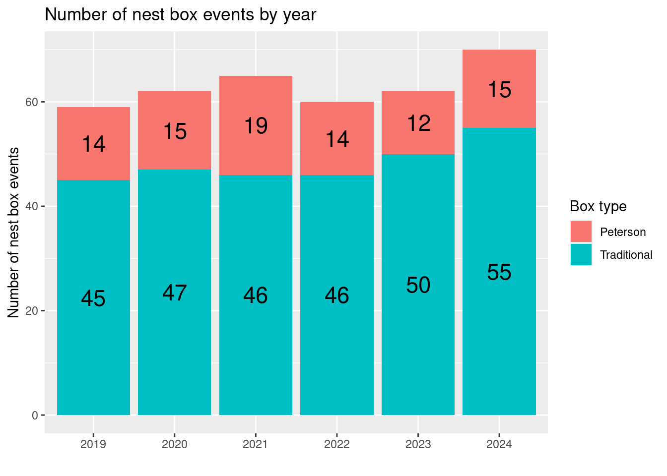
How many boxes were monitored each year?
Let’s start with how many physical boxes we have of each type in the four main parks monitored. Not all of these boxes are active, they are just in the data table. For any query involving site_sf, we use the st_drop_geometry() function to prevent the geometry from showing up in our nice output tables.
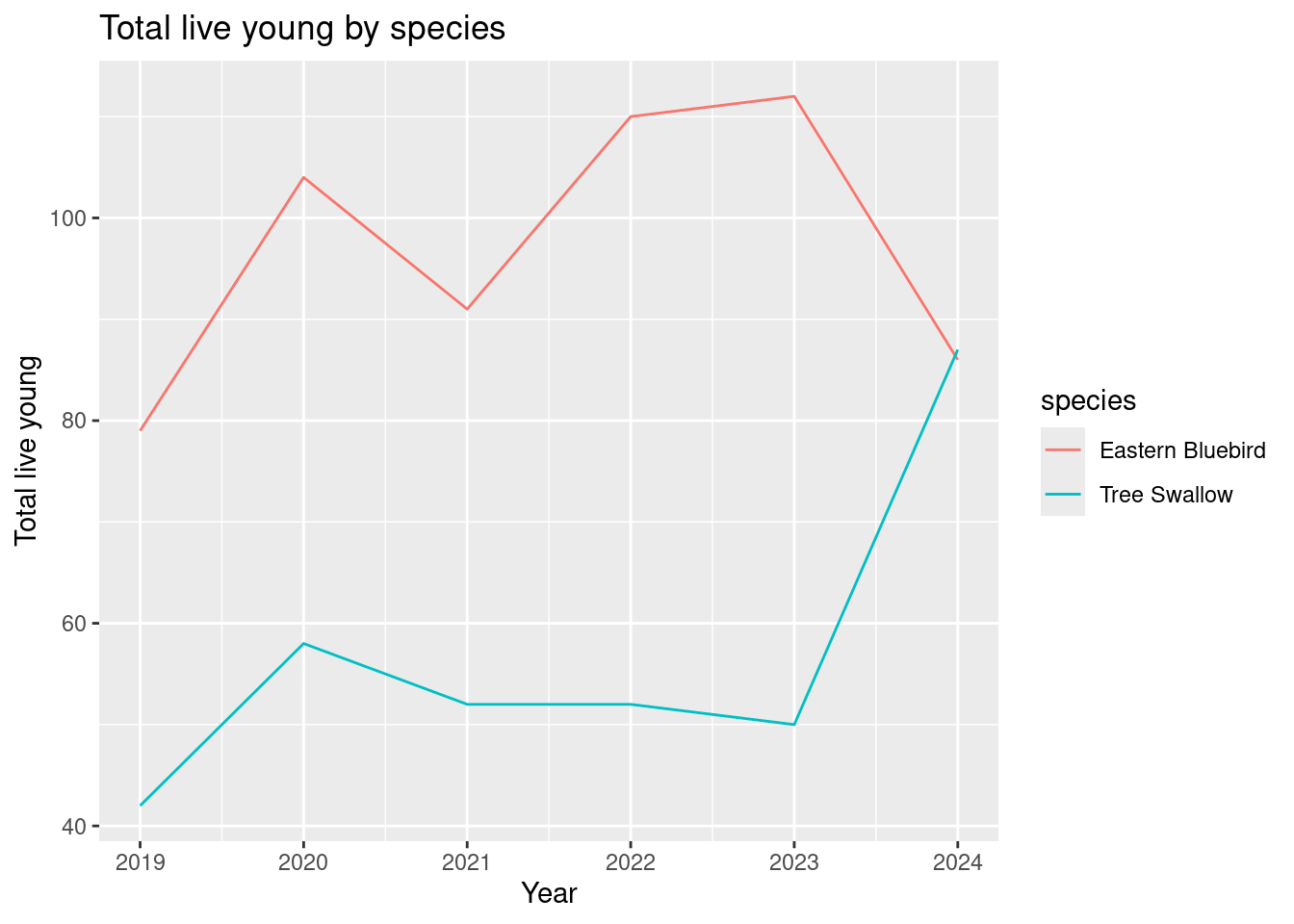
annual_species_counts |>filter(species %in%c("Eastern Bluebird", "Tree Swallow")) |>ggplot() +geom_line(aes(x = site_year, y = tot_live_young, colour = species)) +labs(x ="Year", y ="Total live young", title ="Total live young by species")
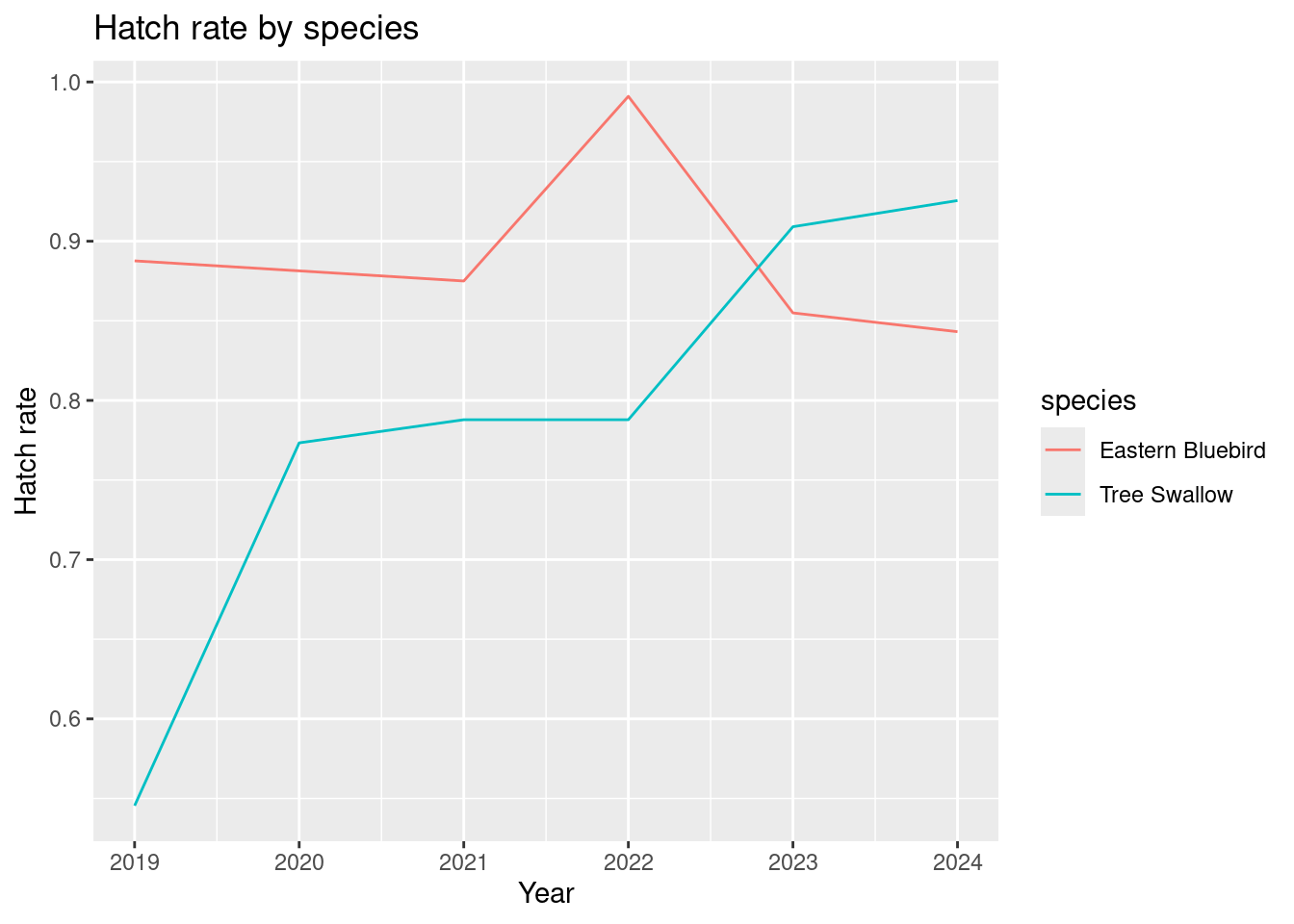
Hatch rate
The hatch rate is the total number of live young divided by the max clutch size observed during the nesting event.
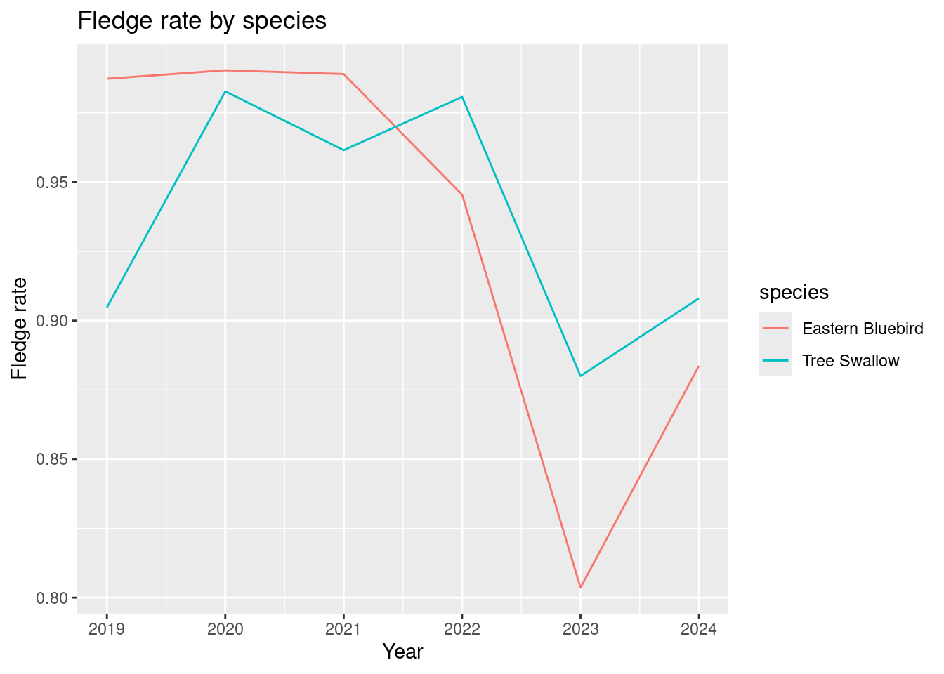
annual_species_counts |>filter(species %in%c("Eastern Bluebird", "Tree Swallow")) |>ggplot() +geom_line(aes(x = site_year, y = overall_fledge_rate, colour = species)) +labs(x ="Year", y ="Fledge rate", title ="Fledge rate by species")
We’ll stop here for now. In the next installment we’ll look to see if there are differences in nesting success in Peterson boxes versus the traditional boxes.
Citation
BibTeX citation:
@online{isken2025,
  author = {Isken, Mark},
  title = {Analyzing {NestWatch} Data with {R}},
  date = {2025-03-01},
  url = {https://bitsofanalytics.org/posts/nestwatch-data-analysis/analyzing_nestwatch_data_r.html},
  langid = {en}
}