library(dplyr)    # General data wrangling

library(sf)       # Simple features such as points, lines, polygons
library(terra)    # Using raster data

library(maptiles) # Fetch map data from places like OpenStreetMap

library(ggplot2)  # Is capable of mapping through geom_sf()
library(ggmap)    # Fetch map data and plot it
library(tidyterra) # Use tidyverse and ggplot2 with terra ojects
library(tmap)     # Static and interactive maps
library(mapsf)    # Static plotting of raster and vector data
library(leaflet) # Interactive mapsHello world maps in R using both raster and vector data
Mapping nest box locations in a nature park
R
geonewb
mapping
geocomputation
birding
nestwatch
Recently I’ve done a bunch of geonewb posts focusing on learning about geospatial analysis using Python. While I’ve barely scratched the surface, I decided to simultaneously explore the same topic using R. I find it helpful to conceptually map (no pun intended) between Python and R packages for doing similar tasks.
A bunch of years ago I did do a post on using ggmap for a simple plot of the state of Michigan (raster data) with dots showing the location and relative size of our state parks (vector data). At the time, one could use ggmap::get_map() to download raster basemaps from Google with no API. Those days are over. Similarly, the terms of use for Open Street Map don’t allow for the get_map() function to use OSM as a source of data for ggmap see Do not use OpenStreetMap export endpoint #117. More importantly, the software landscape has continued to evolve with new packages such as sf, terra and tmap.
Let’s start out with a super simple project and use that to provide a framework for learning basic geocomputation in R. I used the word geocomputation purposefully as one of the first resources I stumbled across in doing this project is the Geocomputation with R (GCwR) online book. It’s a terrific resource. I particularly liked the inclusion of a detailed historical perspective on the geospatial landscape in R. Chapter 9 on Making Maps with R introduces a number of R packages for creating a wide variety of map types. We will see a few of these packages in this brief tutorial.
Ok, let’s start our “Hello World” level project.
Mapping blue bird nest box locations
One of the programs run by the Cornell Lab of Ornithology is known as NestWatch.
NestWatch is a nationwide nest-monitoring program designed to track status and trends in the reproductive biology of birds.
Our local birding group has participated in this program for a number of years. One member has built numerous bluebird boxes and our group has installed and monitored these nest boxes for a number of years. The location (longitude and latitude) of each box is recorded in a database and our goal is to construct a very simple map having:
- a background basemap showing roads and park boundaries,
- each bluebird box shown on the map as a symbol,
- the style of the box symbols should depend on the type of nest box - traditional vs Peterson.
Read the data into a dataframe from a RDS file.
site_df <- readRDS('data/site_df.rds')List key columns for the nest boxes.
site_df %>%
  select(site_name, latitude, longitude, box_type)
# A tibble: 50 × 4
site_name latitude longitude box_type
<chr> <dbl> <dbl> <fct>
1 Kestrel Box 42.8 -83.1 Kestrel
2 DTLP_K1 42.8 -83.1 Traditional
3 CIP_K2 42.8 -83.1 Kestrel
4 PCT01 42.7 -83.2 Traditional
5 PCT02 42.7 -83.2 Traditional
6 PCT04 42.7 -83.2 Traditional
7 PCT03 42.7 -83.2 Traditional
8 PCT05 42.7 -83.2 Traditional
9 PCT06 42.7 -83.2 Traditional
10 PCT07 42.7 -83.2 Traditional
# ℹ 40 more rowsCount the number of nest boxes by box type.
site_df %>%
  group_by(box_type) %>%
  count()
# A tibble: 3 × 2
# Groups: box_type [3]
box_type n
<fct> <int>
1 Kestrel 2
2 Peterson 9
3 Traditional 39Raster and vector data for our map
As the background for the map, we want to show roads, park boundaries and other standard street map elements. This can’t simply be an image file as we also need geographic, or spatial, awareness to be able to overlay the nest box location symbols. As you are likely aware, the two major classes of spatial data are vector and raster. Vector data consists of points, lines, polygons and generalizations of them. Raster data is based on a matrix of cells overlaid on a surface.
Imbueing these data types with geographic awareness involves things like choosing a specific coordinate reference system, or CRS (i.e. the meaning of the X and Y coordinates), an underlying model of our earth and a way of projecting 3D objects onto a 2D surface. See Chapters 2 and 7 of the Geocomputation with R book for the details. The QGIS (a free and open source desktop GIS package) documentation also has a good overview of these topics as does the online text Introduction to GIS and Spatial Analysis by Manuel Gimond.
Our underlying base map will be based some sort of raster file and the nest box points will be vector data based on the latitude and longitude columns of site_df. Two questions immediately arise:
- Where do we get a raster file for the base map of the area we are interested in?
- How do we give true spatial awareness to the
site_dfdataframe?
Let’s tackle the second question first.
Simple features and creating a geographically aware dataframe
While we have longitude and latitude fields in our dataframe, site_df is not really a spatially aware object. In order to make it easy to do spatial related queries, computations and visualizations, we need to fortify it with some spatial powers. To do this we’ll use the sf package.
A package that provides simple features access for R.
With sf we can represent simple planar features such as points, lines and polygons (and multi versions of these things) and manipulate them in dataframes or tibbles. In the Python world we used the GeoPandas package (which relied on the shapely package). Simple features is a general concept supported in many geocomputational tools including things like QGIS and PostGIS.
Before diving into using sf with our longitude/latitude fields, let’s create some basic things like points, lines, and polygons on an Cartesian X-Y coordinate plane. The example below is based on the sf docs with a bit of commentary more detailed exploration added.
# Create a numeric matrix
p <- rbind(c(3.2,4), c(3,4.6), c(3.8,4.4), c(3.5,3.8), c(3.4,3.6), c(3.9,4.5))
# Convert the matrix to a MULTIPOINT object
(mp <- st_multipoint(p))
MULTIPOINT ((3.2 4), (3 4.6), (3.8 4.4), (3.5 3.8), (3.4 3.6), (3.9 4.5))class(mp)[1] "XY" "MULTIPOINT" "sfg" So, mp is an sfg object. These sfg objects could be store in an sfc object as a column in a spatially aware dataframe. It also looks like this specific object instance is a MULTIPOINT - of course it is, we used st_multipoint. I’m guessing that the "XY" means that its two dimensional with X and Y dimensions (no Z or M dimensions). The st_multipoint object does not have a CRS associated with it. That will happen later when we create an sf dataframe. We can use sf::plot, which just extends base::plot to visualize the points.
plot(mp, pch = 16, col = "blue", bg = "blue",
     axes = TRUE, xlab = "X", ylab = "Y")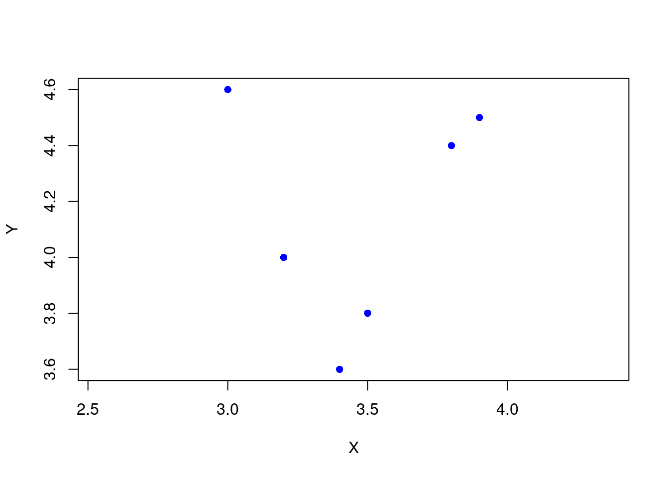
What about lines? They are just ordered collections of POINT objects.
s1 <- rbind(c(0,3), c(0,4), c(1,5), c(2,5))
(linestring <- st_linestring(s1))
LINESTRING (0 3, 0 4, 1 5, 2 5)plot(linestring, col = "blue", axes = TRUE, xlab = "X", ylab = "Y")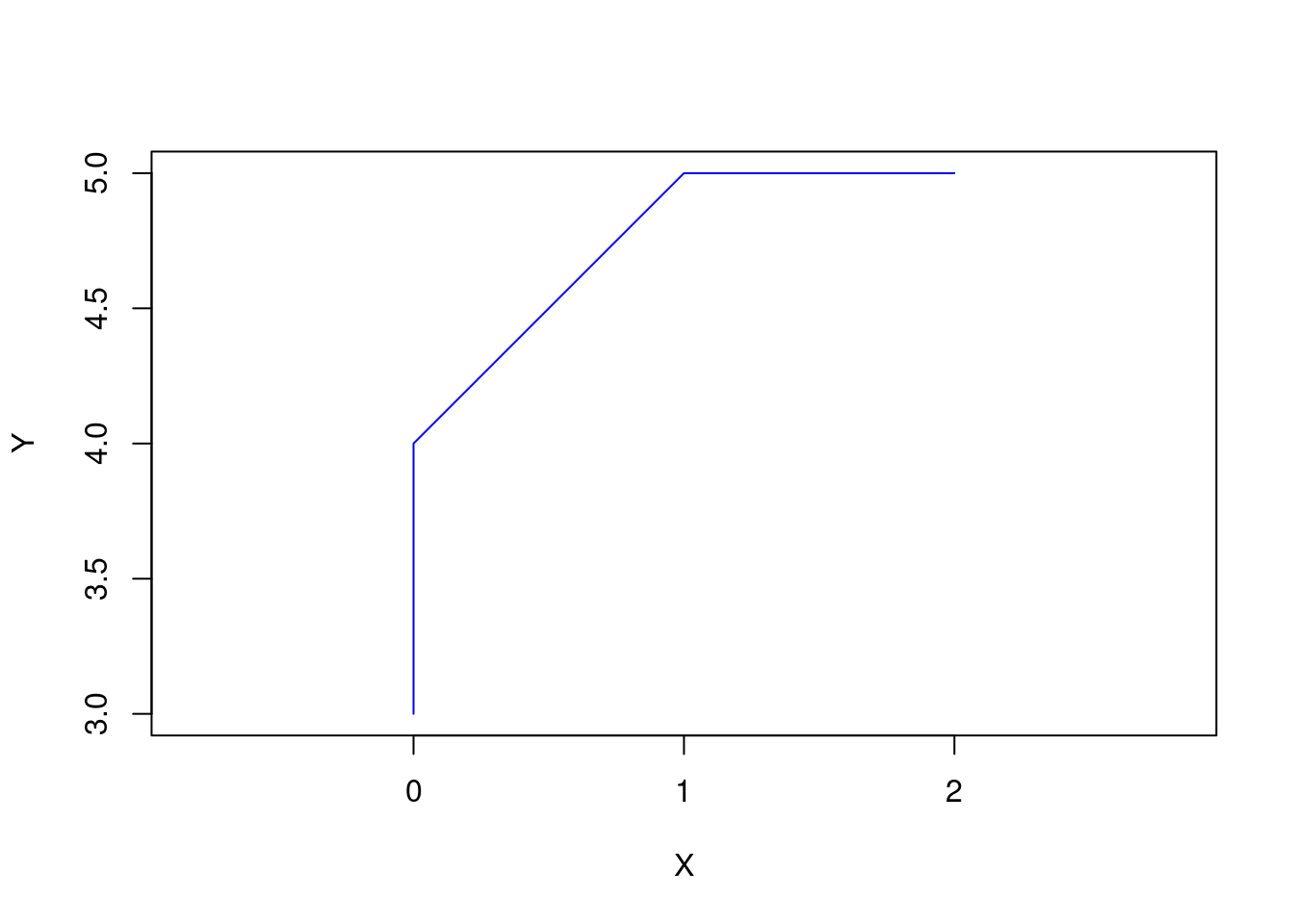
You can create a MULTILINESTRING from a collection of lines in a list.
s2 <- rbind(c(0.2,3), c(0.2,4), c(1,4.8), c(2,4.8))
s3 <- rbind(c(0,4.4), c(0.6,5))
(mls <- st_multilinestring(list(s1, s2, s3)))
MULTILINESTRING ((0 3, 0 4, 1 5, 2 5), (0.2 3, 0.2 4, 1 4.8, 2 4.8), (0 4.4, 0.6 5))plot(mls, col = "blue", axes = TRUE, xlab = "X", ylab = "Y")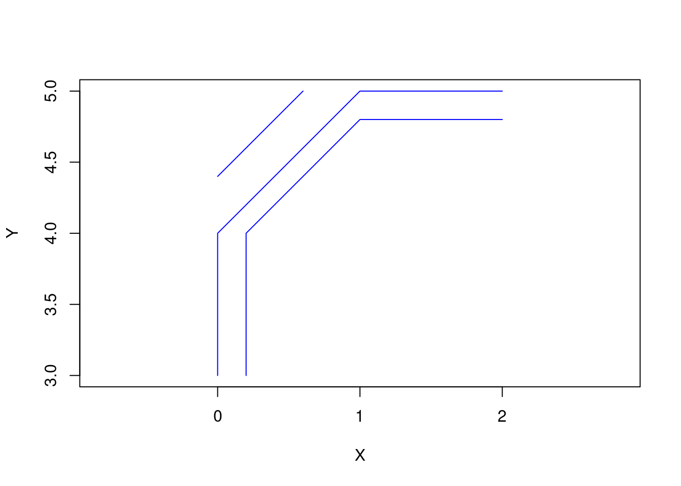
POLYGON objects are just a set of ordered points that start and end with the same point.
p1 <- rbind(c(0,0), c(1,0), c(3,2), c(2,4), c(1,4), c(0,0))
pol1 <-st_polygon(list(p1))
plot(pol1, axes = TRUE, xlab = "X", ylab = "Y")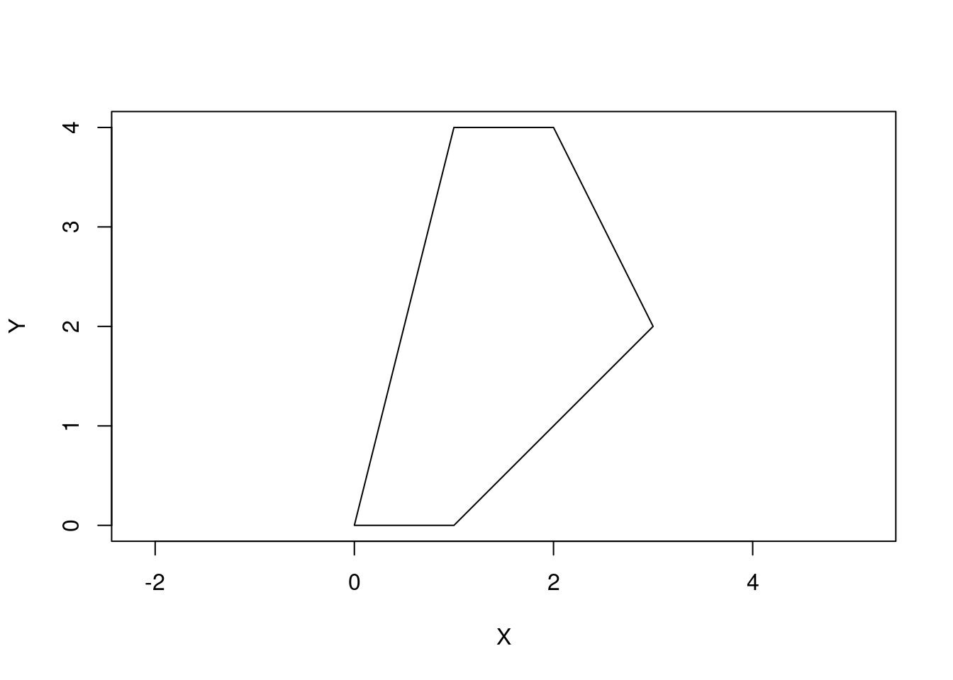
We can make holes or islands by using a few polygons.
p2 <- rbind(c(1,1), c(1,2), c(2,2), c(1,1))
pol2 <-st_polygon(list(p1, p2))
plot(pol2, axes = TRUE, xlab = "X", ylab = "Y")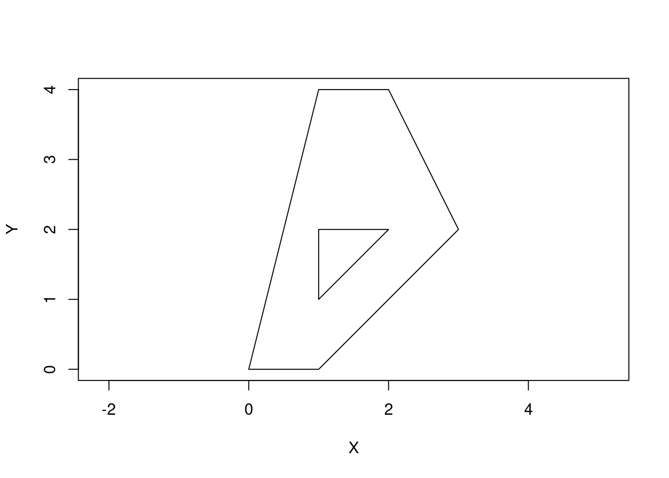
To represent a collection of polygons, use MULTIPOLYGON.
p3 <- rbind(c(3,0), c(4,0), c(4,1), c(3,1), c(3,0))
p4 <- rbind(c(3.3,0.3), c(3.8,0.3), c(3.8,0.8), c(3.3,0.8), c(3.3,0.3))[5:1,]
p5 <- rbind(c(3,3), c(4,2), c(4,3), c(3,3))
(mpol <- st_multipolygon(list(list(p1, p2), list(p3, p4), list(p5))))
MULTIPOLYGON (((0 0, 1 0, 3 2, 2 4, 1 4, 0 0), (1 1, 1 2, 2 2, 1 1)), ((3 0, 4 0, 4 1, 3 1, 3 0), (3.3 0.3, 3.3 0.8, 3.8 0.8, 3.8 0.3, 3.3 0.3)), ((3 3, 4 2, 4 3, 3 3)))plot(mpol, axes = TRUE, xlab = "X", ylab = "Y")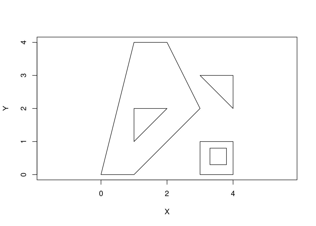
And to create a collection of simple features, we can use a GEOMETRYCOLLECTION.
(gc <- st_geometrycollection(list(mp, mpol, linestring)))GEOMETRYCOLLECTION (MULTIPOINT ((3.2 4), (3 4.6), (3.8 4.4), (3.5 3.8), (3.4 3.6), (3.9 4.5)), MULTIPOLYGON (((0 0, 1 0, 3 2, 2 4, 1 4, 0 0), (1 1, 1 2, 2 2, 1 1)), ((3 0, 4 0, 4 1, 3 1, 3 0), (3.3 0.3, 3.3 0.8, 3.8 0.8, 3.8 0.3, 3.3 0.3)), ((3 3, 4 2, 4 3, 3 3))), LINESTRING (0 3, 0 4, 1 5, 2 5))plot(gc, axes = TRUE, xlab = "X", ylab = "Y")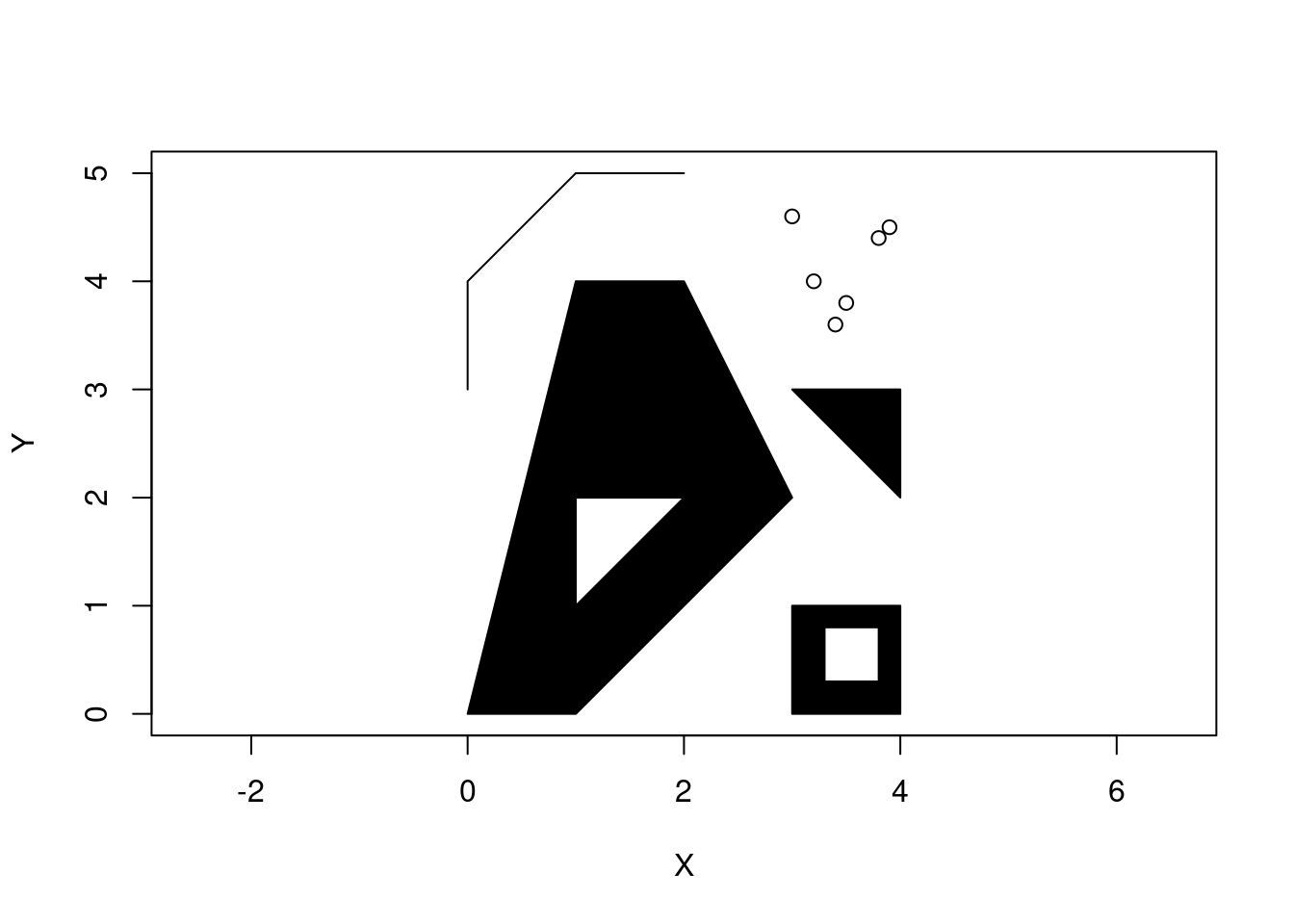
Creating a geodataframe
By creating a column in a dataframe (an sfc object) containing a geometric object (an sfg object) in each row and assigning some sort of CRS, we can get a spatially aware dataframe - a geodataframe you might say (that’s what Python says). The site_df dataframe contains longitude and latitude columns and we can use them with sf::st_as_sf to create a geodataframe. Be careful with the order of longitude and latitude (think X before Y).
site_sf <- st_as_sf(x = site_df,
                    coords = c("longitude", "latitude"),
                    crs = "+proj=longlat +datum=WGS84 +ellps=WGS84 +towgs84=0,0,0")
The "+proj=longlat +datum=WGS84 +ellps=WGS84 +towgs84=0,0,0" is what is known as a PROJ4 string and it contains the parameters of a given CRS. The PROJ library is the thing that does transformations between different coordinate reference systems. The +datum=WGS84 +ellps=WGS84 part specifies which specific ellipsoid model of the earth to use. There are other, simpler, ways to specify the CRS such as using EPSG codes. In this case, crs = 4326 gives us the same CRS as the PROJ4 string and is the familiar long/lat system using the WGS84 earth-centered ellipsoid model.
Under the hood, sf has built in interfaces to key geospatial libraries such as GDAL (reading and writing geographic data files), PROJ (represent and transform projected CRS), and GEOS (geometric operations). It seems that sf interacts directly with these low level libraries instead of using R based wrappers such as rgdal and rgeos. These wrapper libraries are being deprecated as we speak. Depending on whether you are using Windows, Mac or Linux, the GDAL, PROJ, and GEOS libraries may get installed when you install sf or you may need to do some library installation yourself (Linux) - all the details are in the installation section of the sf docs.
Here’s a look at a few important columns of site_sf for one of the parks. Notice that we don’t have to explicitly select the geometry column as it gets displayed automatically just because it is a geodataframe (it’s an sf object). We can use mutate to show a WKT (well known text) representation of each point object - in this case we see the longitude and latitude values for each nest box.
site_sf %>%
  filter(area %in% c('BCNP')) %>%
  select(site_name, box_type) %>%
  mutate(coords_wkt = st_as_text(geometry))
Simple feature collection with 6 features and 3 fields
Geometry type: POINT
Dimension: XY
Bounding box: xmin: -83.15487 ymin: 42.73292 xmax: -83.154 ymax: 42.7351
Geodetic CRS: +proj=longlat +datum=WGS84 +ellps=WGS84 +towgs84=0,0,0
# A tibble: 6 × 4
site_name box_type geometry coords_wkt
* <chr> <fct> <POINT [°]> <chr>
1 BCNP01 Traditional (-83.15468 42.733) POINT (-83.15468 42.733)
2 BCNP02 Peterson (-83.1547 42.73292) POINT (-83.1547 42.73292)
3 BCNP03 Peterson (-83.15487 42.73436) POINT (-83.15487 42.73436)
4 BCNP04 Traditional (-83.15484 42.73442) POINT (-83.15484 42.73442)
5 BCNP05 Peterson (-83.15403 42.73501) POINT (-83.15403 42.73501)
6 BCNP06 Traditional (-83.154 42.7351) POINT (-83.154 42.7351) Plotting geodataframes - sf, ggplot2 and tmap
What happens if we plot the geometry column?
plot(site_sf$geometry, axes = TRUE)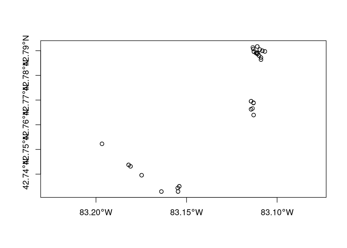
Not the prettiest map, but it’s a start. Since sf::plot is based on the base R plotting system, you might be wondering if we can use ggplot2 to create this same plot - just in a more aesthetically please ggplot style. Yep, you can use geom_sf. Notice that we don’t need to specify the geometry column. Each sf geodataframe has one active default geometry column and that’s the column being used to locate the points on the plot. To plot other geometry columns (gfc objects) just specify them explicitly when using ggplot2 functions.
ggplot() +
    geom_sf(data = site_sf, size = 4, shape = 21, fill = "#3399FF")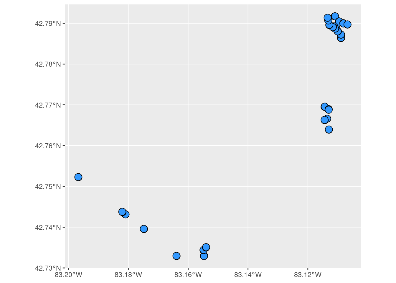
What about other mapping packages like tmap?
- similar in spirit and philosophy to ggplot2 but focused on mapping,
- can make both static and interactive maps via mode setting,
- can handle both vector and raster objects directly.
Let’s figure out how to work with raster files and find a base map for our NestWatch map. Then we’ll use tmap (and try out a few other R mapping packages) to create our map.
Adding a raster base map
We return to our first question - where do we get a raster (or vector) file for the base map of the area we are interested in? Ideally, we’d like a free and open licensed raster map showing things like roads, park boundaries and trails in an aesthetically pleasing manner. We aren’t interested in satellite or aerial images, just a simple static background map on which to overlay the nest box points from site_sf.
Turns out there are several possible sources for a basemap for my use case. From GCwR, 8.2 Retrieving open data talks about general sources and 8.3 Geographic data packages is about R packages providing access to various open map data sources.
Since we want a map of a pretty limited area, any map retrieval function (in any R package or web service) is going to want a specification of our location of interest. Usually this is done either by specifying a longitude/latitude pair or by a bounding box (left/bottom/right/top). To get the values for this map, I just used OpenStreetMap to find the park I was interested in - Bear Creek Nature Park and downloaded the XML file containing the vector data (nodes making up the polygon for the park borders). However, OSM uses its own special data structures for representing vector data and translating it to sf objects is a bit tricky to understand. It’s all explained in this vignette for the osmdata package.
Let’s read that file with the osmdata package.
bcnp_osmdata_sf <- osmdata::osmdata_sf(doc = 'basemaps/bcnp_vector.osm')Error in loadNamespace(x): there is no package called 'osmdata'This error is related to the way that features are represented in OSM and in the downloaded XML file. Let’s not get bogged down and instead look for alternative ways to get a base map.
When I was downloading the XML file from Open Street Map, I grabbed the geographic coordinates for the bounding box of interest.
# left
xmin <- -83.1567
# bottom
ymin <- 42.7314
# right
xmax <- -83.1509
# top
ymax <- 42.7368

bbox <- c(xmin, ymin, xmax, ymax)

# interior point
longitude <- -83.1510
latitude <- 42.7325
Let’s start with ggmap. From the ggmap GitHub repo:
ggmap is an R package that makes it easy to retrieve raster map tiles from popular online mapping services like Google Maps and Stamen Maps and plot them using the ggplot2 framework:
Since ggmap is built on top of ggplot2, you can all of the geom_*’s in ggplot2. There is a qmplot function that is analogous to qplot but with a background map automatically included. The map sources that were originally available via ggmap include Google, Open Street Map (OSM) and Stamen Maps. Unfortunately, due to OSM usage restrictions, it is no longer a valid source for the get_map function. You can learn more about this issue from one of their GitHub issues:
Google Maps needs an API key. I also tried Stamen Maps as the source but got nothing but 404 errors. Let’s try something else. The maptiles package looks promising.
To create maps from tiles, maptiles downloads, composes and displays tiles from a large number of providers (e.g. OpenStreetMap, Stamen, Esri, CARTO, or Thunderforest).
Let’s get the default with just a bounding box specified. The default provider is Open Street Map and we’ll get the entire tile (or tiles) needed to contain the bounding box.
library(maptiles)

bbox_maptiles <- ext(xmin, xmax, ymin, ymax)
bcnp_basemap_osm_default <- maptiles::get_tiles(bbox_maptiles)
This should be a SpatRaster.
bcnp_basemap_osm_defaultclass : SpatRaster
size : 643, 875, 3 (nrow, ncol, nlyr)
resolution : 9.41e-06, 9.41e-06 (x, y)
extent : -83.15826, -83.15003, 42.73087, 42.73692 (xmin, xmax, ymin, ymax)
coord. ref. : lon/lat WGS 84 (EPSG:4326)
source(s) : memory
colors rgb : 1, 2, 3
names : lyr.1, lyr.2, lyr.3
min values : 0, 1, 1
max values : 255, 255, 255Plot it.
plot(bcnp_basemap_osm_default)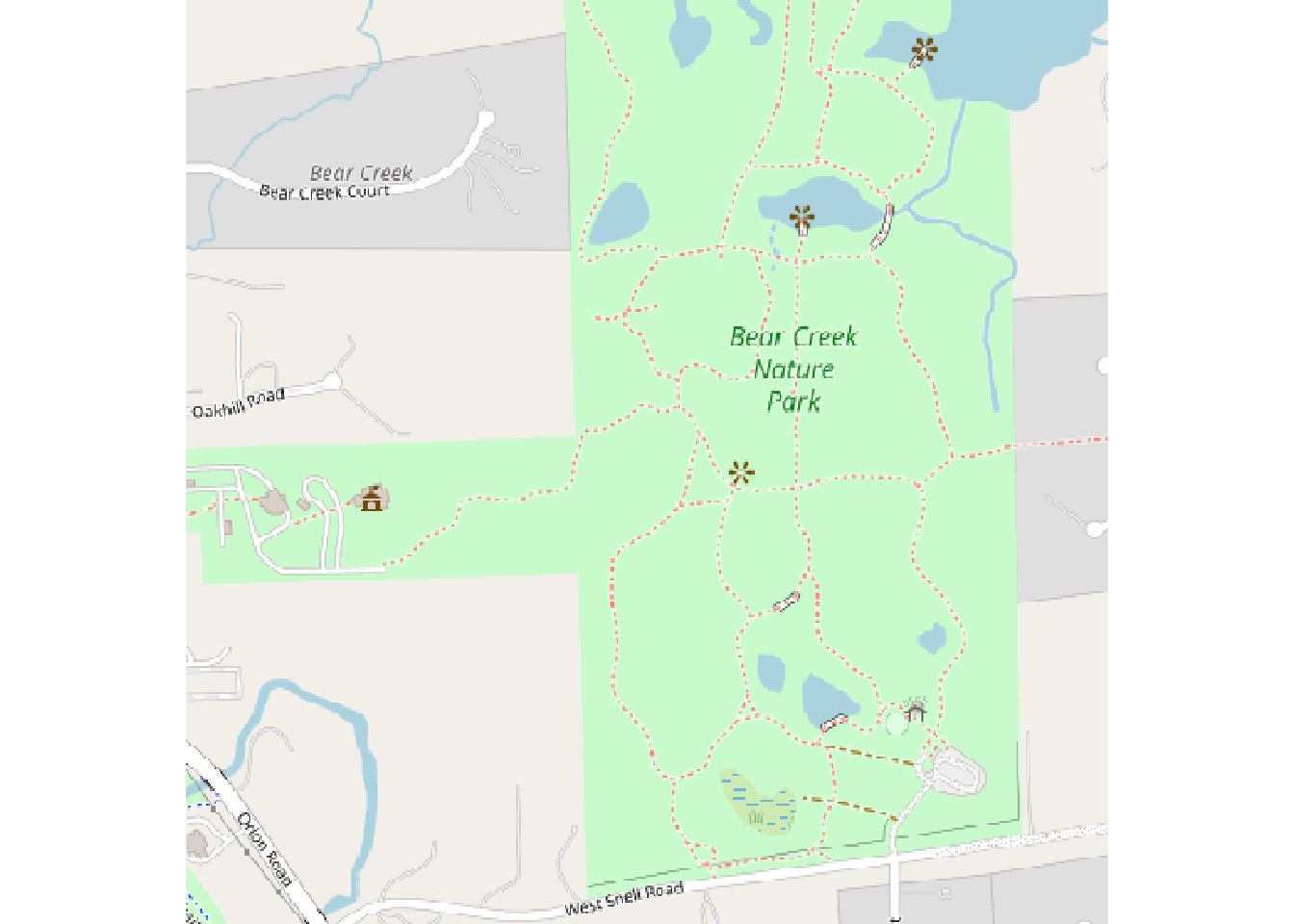
We can either crop it now or we could download with crop = TRUE
bcnp_basemap_osm_default <- crop(bcnp_basemap_osm_default, bbox_maptiles)
plot(bcnp_basemap_osm_default)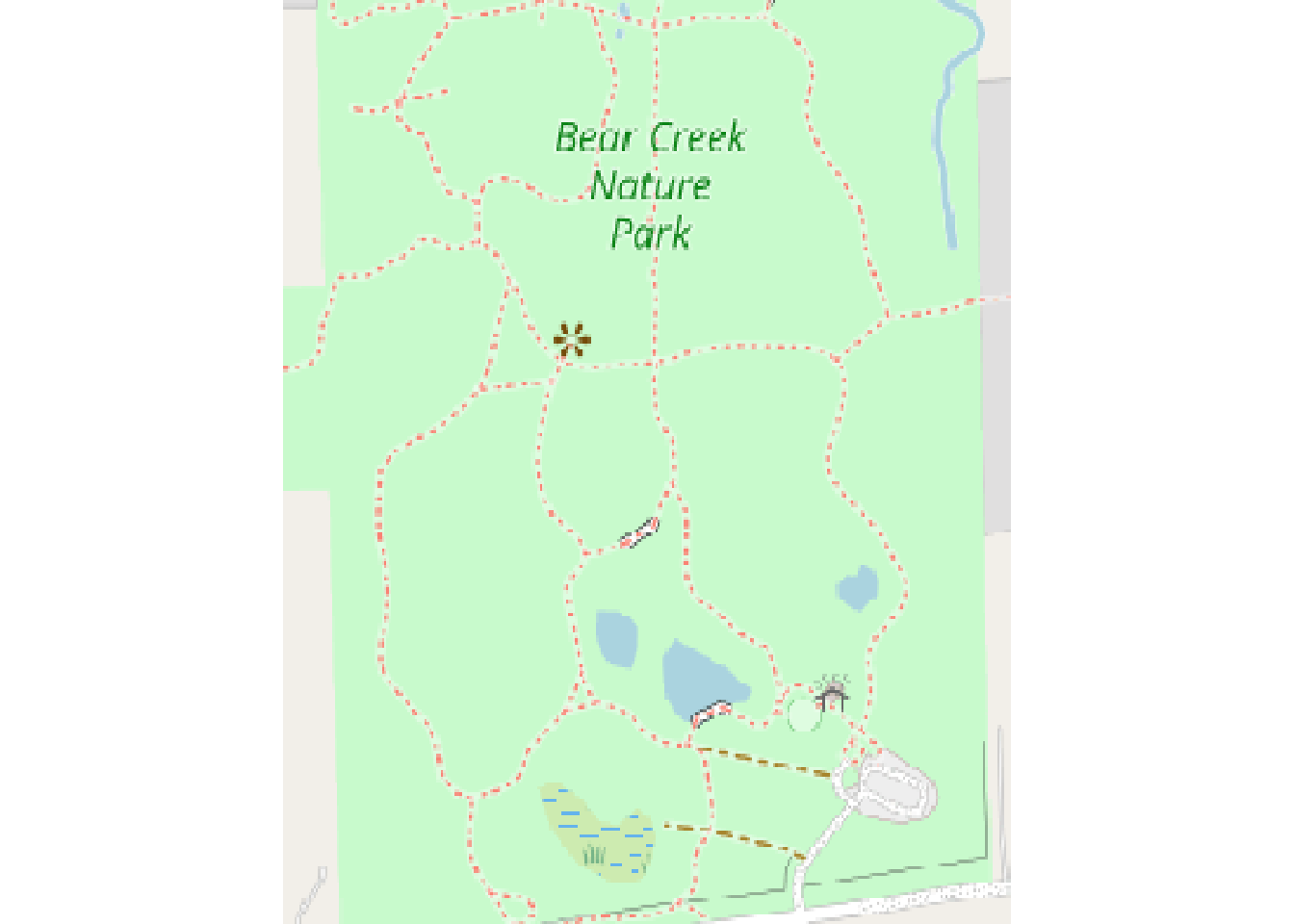
Now let’s overlay the points. We’ll plot the map using terra::plotRGB as well as terra::plot() (which extends base::plot()).
bcnp_points <- site_sf %>%
  filter(area %in% c('BCNP'))

# plot_tiles() is a wrapper for terra::plotRGB()
terra::plotRGB(bcnp_basemap_osm_default)

# Notice the add=TRUE so that points added to previous plot
terra::plot(st_geometry(bcnp_points), add = TRUE,
            pch = 16, col = "#3399FF", bg = "#3399FF")

# Add credit
mtext(text = get_credit("OpenStreetMap"),
      side = 1, line = -1, adj = 0.6, cex = .9,
      font = 3)
Each of the pair of nest boxes consist of one traditional box and one Peterson style box. The point color should correspond to the nest box type. I’m no expert with base plotting, but I’m guessing that the easiest way to do this is to plot separate sets of points for each box type.
bcnp_points_traditional <- site_sf %>%
  filter(area %in% c('BCNP'), box_type == 'Traditional')

bcnp_points_peterson <- site_sf %>%
  filter(area %in% c('BCNP'), box_type == 'Peterson')

# plot_tiles() is a wrapper for terra::plotRGB()
terra::plotRGB(bcnp_basemap_osm_default)

# Notice the add=TRUE so that points added to previous plot
terra::plot(st_geometry(bcnp_points_traditional), add = TRUE,
            pch = 16, col = "#3399FF", bg = "#3399FF")

terra::plot(st_geometry(bcnp_points_peterson), add = TRUE,
            pch = 16, col = "#CC3333", bg = "#CC3333")

# Add credit
mtext(text = get_credit("OpenStreetMap"),
      side = 1, line = -1, adj = 0.6, cex = .9,
      font = 3)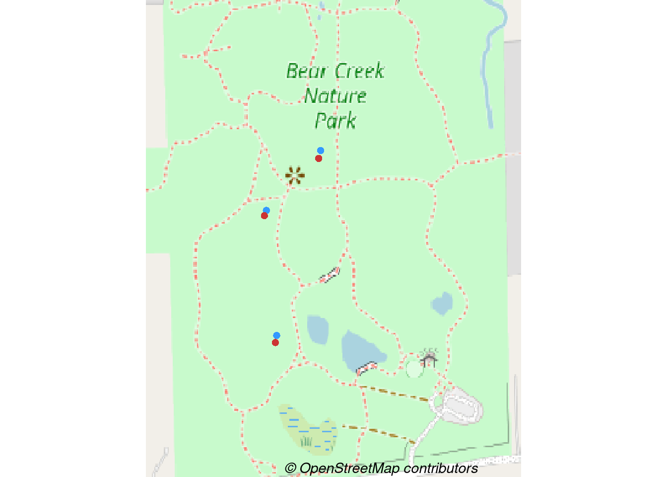
Instead of additional elements to this map, let’s explore other options for making maps from this same data.
Other mapping packages
ggplot2 - yes, it can make maps
As we saw above, the very popular ggplot2 package has some built in mapping capabilities. The geom_sf() function makes it easy to plot simple features such as the nest box points. What about adding the base map?
The tidyterra package provides tidyverse functionality for terra SpatVector and SpatRaster objects. This includes geom_ functions for ggplot2.
library(tidyterra)plot_ggplot <- ggplot() +
geom_spatraster_rgb(data = bcnp_basemap_osm_default) +
geom_spatvector(data = bcnp_points, aes(color = box_type, shape = box_type), size = 3) +
ggtitle("BCNP Nest Box Locations") +
# Need both the following with same name to harmonize the two legends
scale_color_discrete(name="Nest Box Type") +
scale_shape_discrete(name="Nest Box Type")
plot_ggplot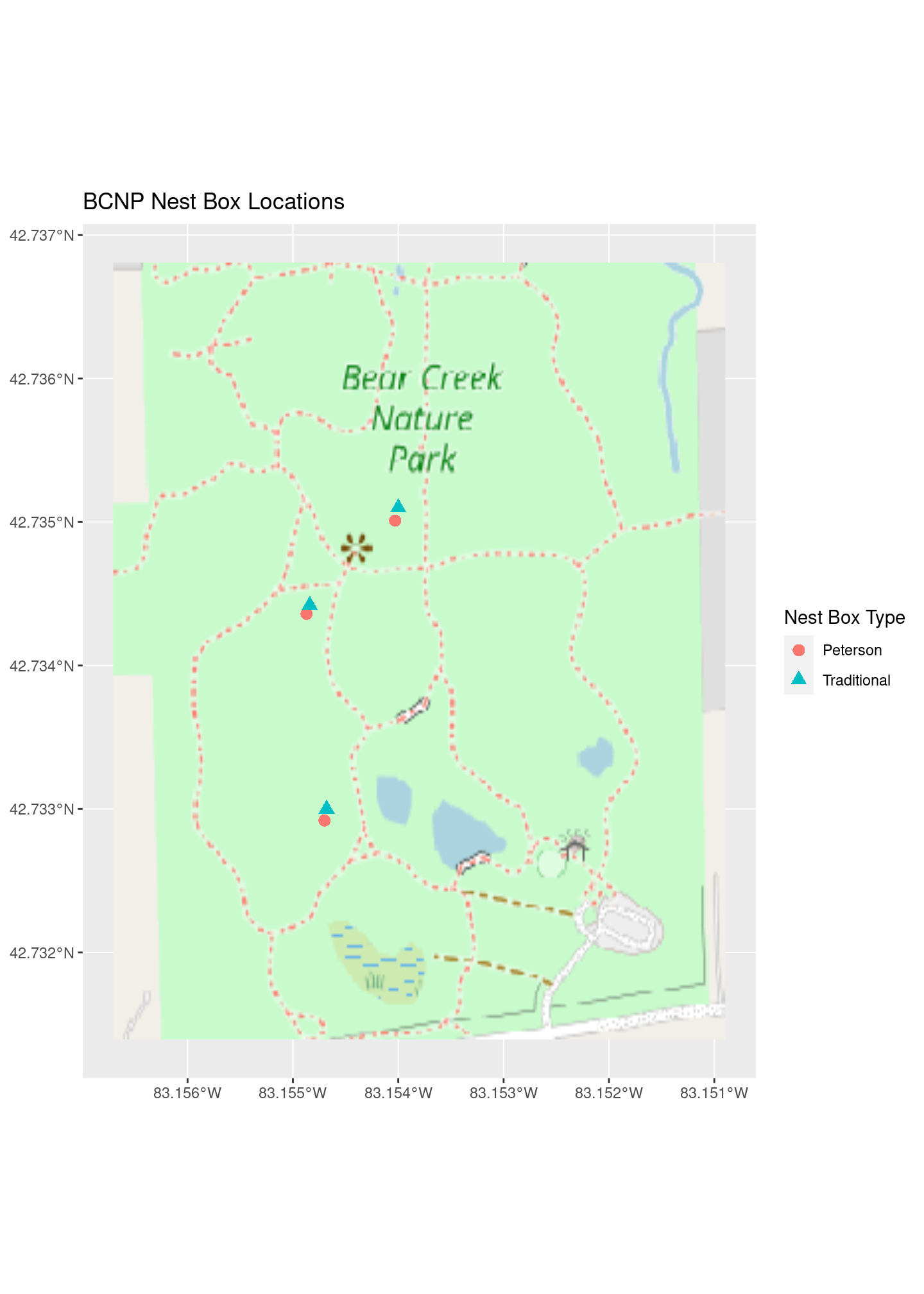
Well, that was easy. Let’s try tmap.
tmap - thematic maps
The tmap package is very ggplot2ish. However, it can create both static and interactive maps by setting its mode via tmap_mode("plot") and tmap_mode("view"), respectively.
The main idea is that each distinct geographic item (e.g. a SpatRaster object) is added to the plot with tm_shape() followed by a series of layer functions that specify the specifics of how to display the item.
library(tmap)# Set mode for static plot
tmap_mode("plot")ℹ tmap modes "plot" - "view"
ℹ toggle with `tmap::ttm()`# Add basemap raster
tm_shape(bcnp_basemap_osm_default) +
tm_rgb() +
# Add nest box points
tm_shape(bcnp_points) +
tm_symbols(col = "box_type", size = .5) +
tm_layout(title = "BCNP Nest Box Locations") +
tm_compass()[v3->v4] `tm_layout()`: use `tm_title()` instead of `tm_layout(title = )`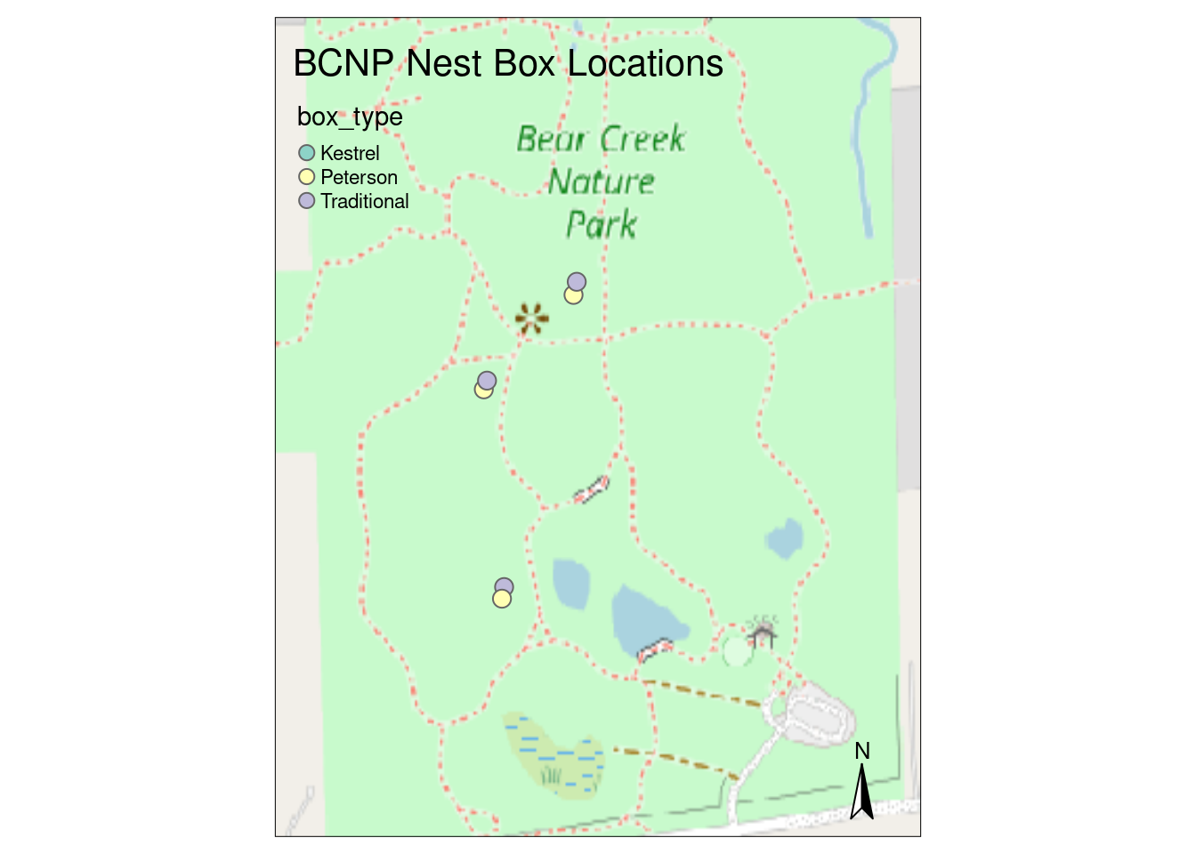
Even though there are no Kestrel boxes, since it’s a level in the box_type column, it shows up in the legend. Also, if I map symbol shape to box_type, we get the double legend result we saw with ggplot2. There are a ton of arguments for the tm_layout() for customizing different aspects of the map layout (e.g. titles, legends, margins, frames, …). These are details for another day.
Overall, it was quite easy to create a basic thematic map with tmap and the similarities in philosophy to ggplot2 should make it attractive to a large number of R users. Additional tmap resources include:
- Getting started tutorial - Hello world for tmap
- Ch 9 of GCwR on Making Maps - tmap featured prominently
- Elegant and informative maps with tmap - draft of online book
- Sneak peek at v4 of tmap - extendability, more aesthetics support
It looks v4 of tmap has some large changes. In addition to the major push for extendability by developers, currently tmap uses stars for raster manipulation and v4 is slated to have better support for terra raster objects. You can install the development version if you want to check it out.
mapsf - another thematic cartography package
The mapsf package is the successor to the cartography package.
Create and integrate thematic maps in your R workflow. This package helps to design various cartographic representations such as proportional symbols, choropleth or typology maps. It also offers several functions to display layout elements that improve the graphic presentation of maps (e.g. scale bar, north arrow, title, labels). mapsf maps sf objects on base graphics.
While tmap seems to be built on ggplot2 for plotting, map_sf relies on extensions to base plotting.
There is a Getting Started tutorial. The package has three main groups of functions:
- Symbology -
mf_mapis the main function which takes as input an sf object, the variables to plot and a plot type. - Map layout - legends, title, scale bar, and more.
- Utilities - other stuff
Between the Getting Started tutorial and the Reference documentation and a little trial and error, it was pretty easy to put the following map together.
library(mapsf)mf_theme("default")The following themes are deprecated:
'default', 'brutal', 'ink', 'dark', 'agolalight', 'candy', 'darkula',
'iceberg', 'green', 'nevermind', 'jsk', and 'barcelona'.
See the Note section in the help page (?mf_theme).# Initialize a map using an sf object (which has an extent)
mf_init(x = bbox_maptiles)
# Add the raster background
mf_raster(bcnp_basemap_osm_default, add = TRUE)
# plot the points, specifying a vector of symbols and colors for the
# levels of the box_type variable.
mf_symb(bcnp_points,
var = "box_type",
pch = c(21,22),
pal = c("red1", "green"),
add = TRUE)
# layout
mf_layout(
title = "BCNP Nest Box Locations",
credits = "Base raster from OpenStreetMap"
)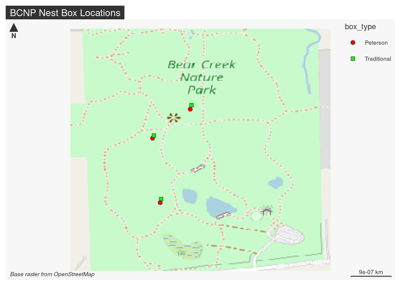
The scale bar cannot be displayed on unprojected (long/lat) maps.leaflet for R - interactive mapping with JS leaflet
The R leaflet package brings Leaflet to R (from JS) so that you can create interactive maps in R.
Leaflet is one of the most popular open-source JavaScript libraries for interactive maps. It’s used by websites ranging from The New York Times and The Washington Post to GitHub and Flickr, as well as GIS specialists like OpenStreetMap, Mapbox, and CartoDB.
What kind of interactivity is possible? This list is from the leaflet docs:
- Interactive panning/zooming
- Compose maps using arbitrary combinations of:
- Map tiles
- Markers
- Polygons
- Lines
- Popups
- GeoJSON
- Create maps right from the R console or RStudio
- Embed maps in knitr/R Markdown documents and Shiny apps
- Easily render spatial objects from the sp or sf packages, or data frames with latitude/longitude columns
- Use map bounds and mouse events to drive Shiny logic
- Display maps in non spherical mercator projections
- Augment map features using chosen plugins from leaflet plugins repository
Let’s recreate our simple Nest Watch map with leaflet. Creating a map with leaflet consists of the same basic steps we’ve seen with the other packages.
- Create a map object based on some extent or bounding box
- Add layers corresponding to the things we want to display on the map
- Show the map
library(leaflet)Let’s create a map by grabbing tiles from OpenStreetMap. Since we want to be able to pan and zoom, we need a dynamic source of map tiles instead of the static raster file we’ve used so far.
m1 <- leaflet() %>%
  addTiles() %>%  # Add default OpenStreetMap map tiles
  addMarkers(lng=longitude, lat=latitude, popup="Bear Creek Nature Park")
m1  # Print the map
We can pan and zoom. We can click the marker to see the pop-up message. Pretty cool. Let’s add the nest boxes. A few things to note about the code below:
- uses the
colorFactor()convenience function to map box type to colors. Note how its return value is used in thecolor =argument toaddCircleMarkers. addCircleMarkersadds circular markers who size remains constant independent of zoom level.- the
values =argument foraddLegendseems to fail if I use a formula such as~box_typeeven though it would seem that the defaultdata = getMapData(map)would inherit thedatafrom the call toaddCircleMarkers. See this GitHub issue.
m2 <- leaflet() %>%
  addTiles() %>%  # Add default OpenStreetMap map tiles
  addMarkers(lng=longitude, lat=latitude, popup="Bear Creek Nature Park")

pal <- colorFactor(c("red1", "green"), domain = c("Peterson", "Traditional"))
m2 <- addCircleMarkers(m2, data=bcnp_points, color = ~pal(box_type),
                       stroke = FALSE, fillOpacity = 0.5, fill = TRUE)
Warning: sf layer has inconsistent datum (+proj=longlat +ellps=WGS84 +towgs84=0,0,0,0,0,0,0 +no_defs).
Need '+proj=longlat +datum=WGS84'm2 <- addLegend(m2, "bottomright", pal = pal, values = bcnp_points$box_type,
title = "Nest Box Types",
opacity = 1)
m2 # Print the mapObviously, this barely scratches the surface of leaflet for interactive maps in R. But, it gives us a good place to stop in this Hello World map post.
mapview - create interactive maps quickly
The R mapview package is all about making it easy to create interactive map visualizations.
mapview provides functions to very quickly and conveniently create interactive visualisations of spatial data. It’s main goal is to fill the gap of quick (not presentation grade) interactive plotting to examine and visually investigate both aspects of spatial data, the geometries and their attributes.
Often a one-liner specifying a vector data source is enough to create an interactive map with (list from the docs):
- a layer control to switch between 5 different background maps
- a scale bar
- information on mouse cursor position and zoom level of the current view
- a zoom-to-layer button to easily navigate to the displayed layer
- popups listing all attribute entries of the respective features (when clicked)
- labels of the feature IDs (when hovered over)
- zoom control buttons provided by the underlying leaflet map
- attribution information of the active map layer in the bottom right corner of the map
Let’s give it a whirl.
library(mapview)mapview(bcnp_points, zcol=c("box_type"))That was impressive! Play around with changing the background layer - if you set it to OpenStreetMap, you’ll see our familiar map. Given that it’s a park, the OpenTopoMap option is a nice one. And, we didn’t even need to go find our own basemaps.
In summary
Having not done mapping in R for quite some time, it was exciting to see how this space has evolved. Key libraries are being updated (or replaced) and there are a multitude of mapping and geocomputation packages. There are also several nice online books for learning about doing geocomputation in R. The parallels with the Python geocomputation community make it pretty easy to wrap your brain around key concepts and the relationship between the various R and Python libraries (e.g. sf and GeoPandas). At this point, I don’t really have a clear preference between R and Python for geocomputation and mapping. I imagine I’ll end up using both quite a bit and plan to keep doing geonewb blog posts that focus on both.
Reuse
Citation
BibTeX citation:
@online{isken2023,
  author = {Isken, Mark},
  title = {Hello World Maps in {R} Using Both Raster and Vector Data},
  date = {2023-04-03},
  url = {https://bitsofanalytics.org/posts/hello_world_mapping_r/hello_world_map_r.html},
  langid = {en}
}
For attribution, please cite this work as:
Isken, Mark. 2023. “Hello World Maps in R Using Both Raster and
Vector Data.” April 3. https://bitsofanalytics.org/posts/hello_world_mapping_r/hello_world_map_r.html.