Using tidymodels for simulation metamodeling

Creating a custom parsnip model

simulation

metamodeling

Author

Mark Isken

Published

February 12, 2023

library(ggplot2)
library(dplyr)
library(tidymodels)
library(MLmetrics)
library(stringr)

Background

A few years ago I wrote a multipart blog series on using R to do simulation metamodeling. The blog posts were inspired by a research project in which I was using queueing inspired feature engineering to try to improve metamodel accuracy and interpretability. The setting for the study was a simulation of inpatient flow through hospital obstetrical units. That study also was an opportunity to learn about the caret package and do some more advanced R programming to automate model fitting and assessment with caret.

Eventually, I redid the entire study in Python and along with my co-authors, Osman Aydas and Yazan Roumani, turned it into a paper that just got accepted in the Journal of Simulation (not sure when it will appear but will update link when it does). For the new study, I rewrote the discrete event simulation model using SimPy and we have released both the model and all of the metamodeling machinery as an open source project so that others can see exactly what we did and to show that everything is reproducible. Here a links to that repo as well as some blog posts I did on using SimPy for patient flow simulation modeling.

In addition to this inpatient flow model, we also created a SimPy model of an outpatient clinic and did another set of metamodeling experiments using it. For the clinic model, I decided to take the opportunity to become more familiar with the the R tidymodels package. I thought it would be a good idea to document some of the challenges and benefits of using tidymodels.

Background on the simulation study

Long ago, when I worked for a large healthcare system, I was involved in a project in which we were building decision support tools for clinic management. Our goal was to have a relatively simple, spreadsheet based tool, that could be used to assess the performance implications of various combinations of key clinic demand and resource related variables. For, example, we wanted to be able to see how increasing the number of patients scheduled in a four hour clinic block or the number of exam rooms per physician would impact things like patient wait times, resource utilization, and the length of time needed to care for all of the patients (since running the clinic past the scheduled closing time resulted in undesirable staffing related consequences and costs).

We developed a discrete event simulation model and ran a series of experiments in which we systematically varied key inputs and tracked key performance measures. Here’s a flow chart for which the simulation model was developed:

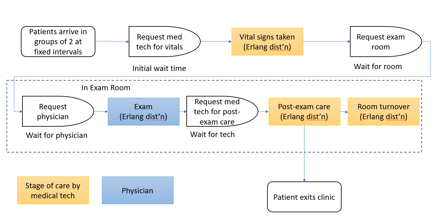
The experimental design included the following input variables as their associated levels:

number of medical technicians (2, 3, 4, 5)
number of exam rooms per physician (1, 2, 3)
mean number of minutes to complete the vital signs portion of the exam by the support staff (6, 9, 12 minutes)
mean number of minutes to complete the exam by the physician (10, 15, 20 mins)
the coefficient of variation squared of the exam time (1.0, 0.5, 0.2)
mean number of minutes to complete post-exam portion of the visit by the support staff (2, 5, 8 minutes)
number of patients in the 4 hour clinic session - patients arrive in groups of two at fixed intervals based on number of total patients. The 5 arrival levels depend on the exam time mean:
- 10 min: 32, 36, 40, 44, 48 patients
- 15 min: 24, 28, 32, 36, 40 patients
- 20 min: 16, 20, 24, 28, 32 patients

The design above leads to 4860 scenarios that were simulated.

The key performance measures (output variables) were:

initial wait time for patient to see med tech for vital signs
mean time until patient saw physician to start exam
mean total time in clinic for the patient
end of the clinic day time

We then developed an Excel based tool that simply did “table lookups” to create plots that showed how the performance measures varies across the levels of the input variables. That original study was then followed by a research project into simulation metamodels for this same clinic experiment. That led to a presentation at the INFORMS 2006 Annual Conference.

Now I am revisiting this same scenario again for this current paper. However, now our goal is to see how queueing inspired feature engineering can improve various simulation metamodeling approaches such as polynomial regression, cubic splines, and random forests. In addition, a nonlinear queueing based power model was also developed - it has far few parameters than the polynomial or spline models and is much more transparent than any of the other modeling approaches.

I entirely rewrote the simulation model in Python (using SimPy) as well as all of the data input machinery for the metamodeling. Then, since I’ve been wanting to explore the tidymodels R package, I used R for the modeling fitting and output analysis. The simulation model can be found at my op_clinic repo.

In this blog post, I’m just going to focus on using the tidymodels package for model fitting and evaluation. We’ll consider a pretty straightforward case - the polynomial regression model, as well as a more complicated case - the nonlinear power model. The complicating factor in using tidymodels for the nonlinear model is that the nls() function is not yet supported as a built in model engine in tidymodels for general nonlinear regression modeling.

About the queueing inspired terms

In the OB patient flow metamodels featured in my previous blog posts, the queueing inspired terms were things related to steady state analysis of the tandem queueing system and relied on things like overall resource load and utilization and steady state queueing results for \(M/G/s\) queueing systems. In contrast, this outpatient modeling problem involves transient analysis (a 4hr clinic block) of a system in which a finite number of scheduled patients arrive for care. Thus, steady state results are not relevant and we can (and do) intentionally overload the system since there are a finite number of patients who will eventually go through the clinic. Obviously, the more you overload the system, the longer the patient wait times and the longer the system has to operate beyond the 4 hour planned end of the day to clear all of the patients.

So, the queuing inspired features for this problem uses known results for mean wait time in transient \(D/M/1\) queues (deterministic arrivals, exponentially distributed service times and a single server). In addition, staff, room and physician offered utilization terms were also included. Unlike in the steady state based scenario of the OB patient flow model, these terms could be greater than 1 (again, an overloaded system). All of the feature engineering was done as part of the Python simulation output analysis. The result is a csv file, xy_q.csv that contains all of the base inputs, queueing related features, and output measures. Our paper (link forthcoming when it’s eventually published, we hope) has all the details.

Let’s dive into tidymodels.

Overview of the analysis with tidymodels

Let’s just focus on one of the performance measures - initial wait time for patient to get staff to begin the clinic care process.

For this blog post we’ll fit three totally different types of metamodels:

polynomial regression
nonlinear multiplicative power model based on queueing inspired features
random forest

For the polynomial models, I was able to use the tidymodels package to create workflows that made it easy to fit a model using repeated k-crossfold resampling and then compute RMSE and an actual vs predicted plot for each model. The Tidy Modeling with R online book by Kuhn and Silge provides a very good introduction to the tidymodels package and how its consitutient packages can be used for different parts of the modeling process.

For those who have used the scikit-learn package in Python, tidymodels will feel familiar except that different parts of the modeling process are handled by different packages under the tidymodels meta-package:

“empty” model objects are created (parsnip)
adding model formulas and various preprocessing steps are done by creating a recipe (recipes)
resampling schemes such as k-crossfold validation or bootstrapping (rsample)
hyperparameter tuning (tune and dials)
model fitting (parsnip and tune)
model predictions (parsnip)
model assessment (yardstick and tune)
put it all together into a modeling workflow, similar to a pipeline in scikit-learn (workflows)

While the presence of so many different packages can be daunting at first, by loading tidymodels you get access to all of the packages. The details of which package does what became very important for this project when we needed to do some deep digging into the API and even the source code to figure out where things were going awry. More on this later.

Reading in of the full input-output dataset

First read in the matrix that contains all possible predictors as well as all possible target variables. Note that some of the predictors are the queueing inspired terms and others are the base inputs used in the simulation experimental design.

xy_q <- read.csv('data/xy_q.csv')

str(xy_q)

'data.frame':   4860 obs. of  32 variables:
 $ patients_per_clinic_block: int  32 36 40 44 48 24 28 32 36 40 ...
 $ num_med_techs            : int  2 2 2 2 2 2 2 2 2 2 ...
 $ num_rooms                : int  2 2 2 2 2 2 2 2 2 2 ...
 $ num_rooms_per_provider   : int  1 1 1 1 1 1 1 1 1 1 ...
 $ num_physicians           : int  2 2 2 2 2 2 2 2 2 2 ...
 $ vitals_time_mean         : int  6 6 6 6 6 6 6 6 6 6 ...
 $ vitals_time_cv2          : num  0.2 0.2 0.2 0.2 0.2 0.2 0.2 0.2 0.2 0.2 ...
 $ exam_time_mean           : int  10 10 10 10 10 15 15 15 15 15 ...
 $ exam_time_cv2            : num  1 1 1 1 1 1 1 1 1 1 ...
 $ post_exam_time_mean      : int  2 2 2 2 2 2 2 2 2 2 ...
 $ post_exam_time_cv2       : num  0.5 0.5 0.5 0.5 0.5 0.5 0.5 0.5 0.5 0.5 ...
 $ room_turnover_time_mean  : num  2.5 2.5 2.5 2.5 2.5 2.5 2.5 2.5 2.5 2.5 ...
 $ room_turnover_time_cv2   : num  0.143 0.143 0.143 0.143 0.143 ...
 $ off_util_staff           : num  0.7 0.787 0.875 0.963 1.05 ...
 $ off_util_physician       : num  0.667 0.75 0.833 0.917 1 ...
 $ off_util_room            : num  0.967 1.087 1.208 1.329 1.45 ...
 $ staff_eff_ia_time_mean   : num  15 13.3 12 10.9 10 ...
 $ staff_eff_svc_time_mean  : num  10.5 10.5 10.5 10.5 10.5 10.5 10.5 10.5 10.5 10.5 ...
 $ staff_eff_svc_time_cv2   : num  0.419 0.419 0.419 0.419 0.419 ...
 $ exam_eff_ia_time_mean    : num  15 13.3 12 10.9 10 ...
 $ exam_eff_svc_time_mean   : num  27.1 32.8 40.1 49.4 60.6 ...
 $ exam_eff_svc_time_cv2    : num  1.19 1.06 1.06 1.09 1.11 ...
 $ mean_wait_i_dm1          : num  6.88 9.99 14.02 19.02 25.03 ...
 $ mean_wait_p_dm1          : num  5.68 8.27 11.63 15.88 21.05 ...
 $ mean_wait_r_dm1          : num  17.6 44.4 92.4 162.6 256 ...
 $ mean_wait_rp_dm1         : num  23.3 52.7 104 178.5 277 ...
 $ mean_wait_i              : num  0.359 0.44 0.544 0.622 0.959 ...
 $ mean_wait_r              : num  7.85 12.99 28.72 35.2 52.19 ...
 $ mean_wait_p              : num  0 0 0 0 0 0 0 0 0 0 ...
 $ mean_wait_rp             : num  7.85 12.99 28.72 35.2 52.19 ...
 $ mean_time_in_system      : num  27.3 32.3 48.8 54.5 72.6 ...
 $ mean_eod                 : num  267 274 306 317 356 ...

The output (dependent) variables, or performance measures, are the last 6 in the list above. We won’t be using all of the input variables in the study for the paper as not all are relevant for the mean_wait_i (“i” for initial) variable we’ll be focusing on.

Details on data partitioning

Create in design and out of design dataframes

As described above, there are a total of 4860 scenarios and within those there are 5 different levels of number of patients per clinic session. In addition to assessing how accurate the various models are within the confines of the experimental design, I thought it would also be interesting to assess their relative peformance in extrapolation beyond the experimental design. So, I decided to treat the highest arrival rate level as the “out of design” holdout set. These scenarios correspond to every 5th row in the the xy_q dataframe.

Create sequence of row numbers to include in the out of design set and the in design set.

ood_rows <- seq(5, 4860, 5)
design_rows <- setdiff(seq(1, 4860,1), ood_rows)

Now subset the main dataframe to create the “in design” dataframe and “out of design” dataframe.

xy_q_in <- xy_q[design_rows, ]
xy_q_out <- xy_q[ood_rows, ]

There are 3888 rows in the in design dataframe and 972 rows in the out of design dataframe.

To begin with, we’ll just be focusing on the the in design dataframe, xy_q_in.

Initial split of in_split

The partitioning that we did so far of xy_q into xy_q_in and xy_q_out is for eventually seeing how well the various models can extrapolate beyond the experimental design space. Now, let’s do an initial split of xy_q_in into training and test dataframes. Then we’ll use k-crossfold validation on the training data and eventually do final model comparisons on the test data. The initial_split function is from the rsample package which I describe more in the next section. I’m using the rsample:: form in the function call just to highlight the fact that these functions are from the rsample package - we’ve loaded tidymodels so there’s really no need to do this.

set.seed(23)
# Do the 75/25 split
xy_q_in_split <- rsample::initial_split(xy_q_in, prop = 0.75)
# Create train and test dataframes based on the split
xy_q_in_train <- rsample::training(xy_q_in_split)
xy_q_in_test <- rsample::testing(xy_q_in_split)

k-fold cross-validation on in design scenarios using the rsample package

One of the packages that falls under the tidymodels umbrella is called rsample. As its name suggests, it support various resampling schemes such as bootstrapping and cross-validation.

In a nutshell, the rsample::vfold_cv function creates a dataframe of rsplit objects that contains the dataset partition information for each resampling step (fold and repeat). The user can then fit models and compute errors on each partition and do whatever kind of error metric averaging desired.

I decided to do 10 repeats of 5-fold cross validation.

set.seed(57)
# Number of folds
kfold_number <- 5
# Number of repeats of entire k-fold process
kfold_repeats <- 10

# Create the split object
in_train_splits <- vfold_cv(xy_q_in_train, v = kfold_number, repeats = kfold_repeats)

We can see that in_train_splits is a tibble of vfold_split objects (which are just special case of rsplit objects).

in_train_splits

#  5-fold cross-validation repeated 10 times 
# A tibble: 50 × 3
   splits             id       id2  
   <list>             <chr>    <chr>
 1 <split [2332/584]> Repeat01 Fold1
 2 <split [2333/583]> Repeat01 Fold2
 3 <split [2333/583]> Repeat01 Fold3
 4 <split [2333/583]> Repeat01 Fold4
 5 <split [2333/583]> Repeat01 Fold5
 6 <split [2332/584]> Repeat02 Fold1
 7 <split [2333/583]> Repeat02 Fold2
 8 <split [2333/583]> Repeat02 Fold3
 9 <split [2333/583]> Repeat02 Fold4
10 <split [2333/583]> Repeat02 Fold5
# … with 40 more rows

Here’s how we can access individual split data. The rsample library uses the term analysis data instead of train and assessment data instead of test.

# Get the first resample object
first_resample <- in_train_splits$splits[[1]]
# Peek at train
head(analysis(first_resample))

     patients_per_clinic_block num_med_techs num_rooms num_rooms_per_provider
1156                        32             4         6                      3
2914                        44             5         2                      1
1589                        28             5         6                      3
1903                        24             2         6                      3
569                         28             3         4                      2
2133                        40             3         2                      1
     num_physicians vitals_time_mean vitals_time_cv2 exam_time_mean
1156              2               12             0.2             10
2914              2               12             0.2             10
1589              2                6             0.2             20
1903              2                6             0.2             20
569               2                9             0.2             20
2133              2                9             0.2             10
     exam_time_cv2 post_exam_time_mean post_exam_time_cv2
1156           1.0                   5                0.5
2914           0.2                   5                0.5
1589           1.0                   8                0.5
1903           0.2                   2                0.5
569            1.0                   2                0.5
2133           0.2                   8                0.5
     room_turnover_time_mean room_turnover_time_cv2 off_util_staff
1156                     2.5              0.1428571       0.650000
2914                     2.5              0.1428571       0.715000
1589                     2.5              0.1428571       0.385000
1903                     2.5              0.1428571       0.525000
569                      2.5              0.1428571       0.525000
2133                     2.5              0.1428571       1.083333
     off_util_physician off_util_room staff_eff_ia_time_mean
1156          0.6666667     0.3888889               15.00000
2914          0.9166667     1.6041667               10.90909
1589          1.1666667     0.5930556               17.14286
1903          1.0000000     0.4083333               20.00000
569           1.1666667     0.7145833               17.14286
2133          0.8333333     1.7083333               12.00000
     staff_eff_svc_time_mean staff_eff_svc_time_cv2 exam_eff_ia_time_mean
1156                    9.75              0.4469540              15.00000
2914                    7.80              0.4469540              10.90909
1589                    6.60              0.5274468              17.14286
1903                   10.50              0.4188926              20.00000
569                     9.00              0.4667363              17.14286
2133                   13.00              0.4155455              12.00000
     exam_eff_svc_time_mean exam_eff_svc_time_cv2 mean_wait_i_dm1
1156               28.31571             1.2781330       5.1373286
2914               39.24771             1.7920118       5.8719084
1589               72.35856             4.5544262       0.6727572
1903               55.25698             2.1498538       2.8133543
569                68.13819             5.2083896       2.4523833
2133               61.72793             0.9745578      29.5965876
     mean_wait_p_dm1 mean_wait_r_dm1 mean_wait_rp_dm1 mean_wait_i mean_wait_r
1156        5.678379       0.2374558         5.915835  0.12145435  0.06615067
2914       15.875804     106.2935891       122.169393  0.04530920 56.45996278
1589       41.185808       7.7328543        48.918662  0.01092027  8.06474237
1903       27.943627       1.6566003        29.600227  0.24243105  0.17063897
569        41.185808      25.7387255        66.924533  0.02372471 12.89212641
2133       11.631343     201.6879895       213.319333  1.01295877 74.78263011
     mean_wait_p mean_wait_rp mean_time_in_system mean_eod
1156    2.382189     2.448340            30.18538 262.8861
2914    0.000000    56.459963            83.92953 371.1970
1589   16.301227    24.365969            57.58385 319.3207
1903    9.240288     9.410927            38.58189 272.0874
569    10.966330    23.858456            54.59284 319.7577
2133    0.000000    74.782630           103.74635 406.5454

# Peek at test
head(assessment(first_resample))

     patients_per_clinic_block num_med_techs num_rooms num_rooms_per_provider
3991                        32             3         6                      3
1268                        32             5         2                      1
1958                        32             2         6                      3
2006                        16             2         6                      3
2233                        24             3         4                      2
3953                        32             3         6                      3
     num_physicians vitals_time_mean vitals_time_cv2 exam_time_mean
3991              2               12             0.2             10
1268              2                6             0.2             15
1958              2                9             0.2             15
2006              2                9             0.2             20
2233              2                9             0.2             20
3953              2               12             0.2             15
     exam_time_cv2 post_exam_time_mean post_exam_time_cv2
3991           0.5                   5                0.5
1268           1.0                   5                0.5
1958           0.2                   5                0.5
2006           0.2                   8                0.5
2233           0.2                   5                0.5
3953           0.5                   2                0.5
     room_turnover_time_mean room_turnover_time_cv2 off_util_staff
3991                     2.5              0.1428571      0.8666667
1268                     2.5              0.1428571      0.3600000
1958                     2.5              0.1428571      1.1000000
2006                     2.5              0.1428571      0.6500000
2233                     2.5              0.1428571      0.5500000
3953                     2.5              0.1428571      0.7333333
     off_util_physician off_util_room staff_eff_ia_time_mean
3991          0.6666667     0.3888889                     15
1268          1.0000000     1.5000000                     15
1958          1.0000000     0.5000000                     15
2006          0.6666667     0.3388889                     30
2233          1.0000000     0.6875000                     20
3953          1.0000000     0.4333333                     15
     staff_eff_svc_time_mean staff_eff_svc_time_cv2 exam_eff_ia_time_mean
3991                    13.0              0.4469540                    15
1268                     5.4              0.3867186                    15
1958                    16.5              0.4144845                    15
2006                    19.5              0.4155455                    30
2233                    11.0              0.4144845                    20
3953                    11.0              0.4587043                    15
     exam_eff_svc_time_mean exam_eff_svc_time_cv2 mean_wait_i_dm1
3991               38.48086             0.8543810      15.3024853
1268               47.80331             4.0144639       0.4398748
1958               80.76920             0.9994200      33.4057701
2006               48.63299             0.6357165       8.6701294
2233               58.82556             2.0912196       3.3819381
3953               52.59627             2.3435171       8.2328360
     mean_wait_p_dm1 mean_wait_r_dm1 mean_wait_rp_dm1 mean_wait_i mean_wait_r
3991        5.678379       0.9271693         6.605548  0.90496542  0.07052544
1268       24.863430      85.6364573       110.499888  0.00000000 42.49793207
1958       24.863430      17.3003260        42.163756  5.25727485  1.40778217
2006        9.462865       0.2235870         9.686452  1.87931011  0.00000000
2233       27.943627      10.1332013        38.076828  0.09146909  2.76873372
3953       24.863430       3.3569486        28.220379  0.24323800  2.42631747
     mean_wait_p mean_wait_rp mean_time_in_system mean_eod
3991    1.991905     2.062430            31.77847 260.0836
1268    0.000000    42.497932            68.23150 348.0091
1958    7.753168     9.160950            50.01683 283.9539
2006    1.297761     1.297761            42.44758 257.8852
2233    6.998359     9.767093            44.14195 276.3151
3953   12.107860    14.534178            44.72451 286.2879

Polynomial regression model for initial wait

Now let’s fit a polynomial regression model to try to predict mean_wait_i (the initial wait time experienced by the patient before their vital signs are taken by a medical technician). We want to do repeated k-crossfold resampling to get a sense of how variable the model is when based on different fit datasets. We can do this all quite easily using tidymodels by building workflow objects to properly handle the model fitting and assessment within the context of resampling.

Start by creating an an empty model object of the appropriate type. Since polynomial regression is really just a linear regression model with some added features (powers of inputs) we use the parsnip::linear_reg function - https://parsnip.tidymodels.org/reference/linear_reg.html. Nothing special is needed for fitting a polynomial regression model in R beyond the lm function and we use set_engine to specify this choice for how the regression model should be fit. Technically, lm' is the default engine forlinear_regbut we are just being explicit. While we don't need them here, thelinear_reg` function also includes optional arguments related to regularization.

wait_i_poly_mod <- linear_reg(mode = "regression") %>% 
  set_engine(engine = "lm")

For sckikit-learn users, the above is analogous to:

from sklearn import linear_model
wait_i_poly_mod = linear_model.LinearRegression()

Next we need to create the specific linear regression formula object we want to fit. This first formula only contains basic inputs and does not include any queueing inspired features. This next line of code has nothing to do with tidymodels, it’s just creation of an R formula object.

# Create a formula object. Later we'll use a recipe to generate the polynomial terms.
wait_i_poly_noq_formula <- mean_wait_i ~ patients_per_clinic_block + 
                         num_med_techs +
                         num_rooms + 
                         vitals_time_mean +
                         exam_time_mean +
                         exam_time_cv2 + 
                         post_exam_time_mean

Now we’ll create a recipe object that contains two steps - the formula and the polynomial transforms. Tidymodels uses the recipe package to let you create objects that encapsulate various modeling pre-processing tasks that occur prior to actually fitting the model. A peek at the recipes docs reveals that recipes tries to provide a wide range of pre-processing functionality such as formula specification, imputation, transformations, dummy encoding, and more. There has been some criticism of recipes (and tidymodels in general) in this regard in that it tries to do too much and does it not very well. I haven’t used tidymodels nearly enough to have formed an opinion yet on this point. In scikit-learn, the sklearn.preprocessing package provides functionality that overlaps with the recipes package in R.

In our case, the only pre-processing we need is to specify the base linear model formula and then add in the polynomial terms. We do the latter by using one the many step_* functions available in recipes - step_poly. For step_poly, the default of degree = 2 corresponds to using up to squared terms.

wait_i_poly_noq_recipe <- recipe(wait_i_poly_noq_formula, data = xy_q_in_train) %>% 
  step_poly(patients_per_clinic_block, num_med_techs, num_rooms,
          vitals_time_mean, exam_time_mean, exam_time_cv2, post_exam_time_mean,
          degree = 2)

Now we can combine our model and our recipe into a workflow. This is reminiscent of Pipeline objects in scikit-learn.

# Create a workflow object that uses the model and recipe above
wait_i_poly_noq_wflow <- 
  workflow() %>% 
  add_model(wait_i_poly_mod) %>% 
  add_recipe(wait_i_poly_noq_recipe)

At this point, we still haven’t fit any models nor done any resampling. We have simply set up a resampling scheme through our creation of the in_train_splits variable (a tibble of vfold_split objects) and created a workflow consisting of a model and a pre-processing recipe. Before launching the resampling and fitting process, we can set some resampling control options through the rsample::control_samples function. For example, we can choose to save the out of sample predictions for later analysis or append the workflow object onto its output.

keep_pred <- control_resamples(save_pred = TRUE, save_workflow = FALSE)

Finally, we can pipe our workflow through tune::fit_resamples().

wait_i_poly_noq_results <- 
  wait_i_poly_noq_wflow %>% 
  fit_resamples(resamples = in_train_splits, control = keep_pred)

Now let’s look at the metrics averaged over the 50 splits (10 repeats x 5 folds). Notice that there’s a small standard error on the metrics indicating that there’s not a lot of variability between splits. This is good. The tune::collect_metrics function makes it easy to pull out and consolidate metrics.

collect_metrics(wait_i_poly_noq_results)

# A tibble: 2 × 6
  .metric .estimator  mean     n std_err .config             
  <chr>   <chr>      <dbl> <int>   <dbl> <chr>               
1 rmse    standard   4.86     50 0.0605  Preprocessor1_Model1
2 rsq     standard   0.408    50 0.00304 Preprocessor1_Model1

Now we’ll refit one last model using the entire training set and assess its performance on the in design test data. For this, we use tune::last_fit().

# Do last fit
wait_i_last_poly_noq_results <- last_fit(wait_i_poly_noq_wflow, xy_q_in_split)

What exactly is returned from last_fit()? It’s a one row tibble of tibbles.

wait_i_last_poly_noq_results

# Resampling results
# Manual resampling 
# A tibble: 1 × 6
  splits             id               .metrics .notes   .predictions .workflow 
  <list>             <chr>            <list>   <list>   <list>       <list>    
1 <split [2916/972]> train/test split <tibble> <tibble> <tibble>     <workflow>

There’s only one row and it corresponds to the initial train/test split that was done. From the column names we see that things like the accuracy metrics and final model predictions are tibbles within this container tibble.

collect_metrics(wait_i_last_poly_noq_results)

# A tibble: 2 × 4
  .metric .estimator .estimate .config             
  <chr>   <chr>          <dbl> <chr>               
1 rmse    standard       4.76  Preprocessor1_Model1
2 rsq     standard       0.398 Preprocessor1_Model1

The RMSE on test is slightly smaller than RMSE on train which is unusual but can happen due to randomness.

Let’s plot the actual vs predicted values based on the in design test dataframe. The predictions on the test data based on the model fit by last_fit can be obtained by tune::collect_predictions().

wait_i_last_poly_noq_rmse <- collect_metrics(wait_i_last_poly_noq_results) %>% 
  filter(.metric == 'rmse') %>% 
  pull(.estimate) 

# Grab the predictions on the test data
assess_wait_i_last_poly_noq_results <- collect_predictions(wait_i_last_poly_noq_results)

# Plot actual vs predicted.
assess_wait_i_last_poly_noq_results %>% 
  ggplot(aes(x = mean_wait_i, y = .pred)) + 
  geom_point(alpha = .15) +
  geom_abline(color = "red") + 
  coord_obs_pred() + 
  xlab("Actual mean initial wait time (min)") +
  ylab("Metamodel prediction") +
  ggtitle("Polynomial regression model - no queueing terms") +
  annotate("text", x = 10, y = 40, label = sprintf("RMSE = %8.3f", wait_i_last_poly_noq_rmse))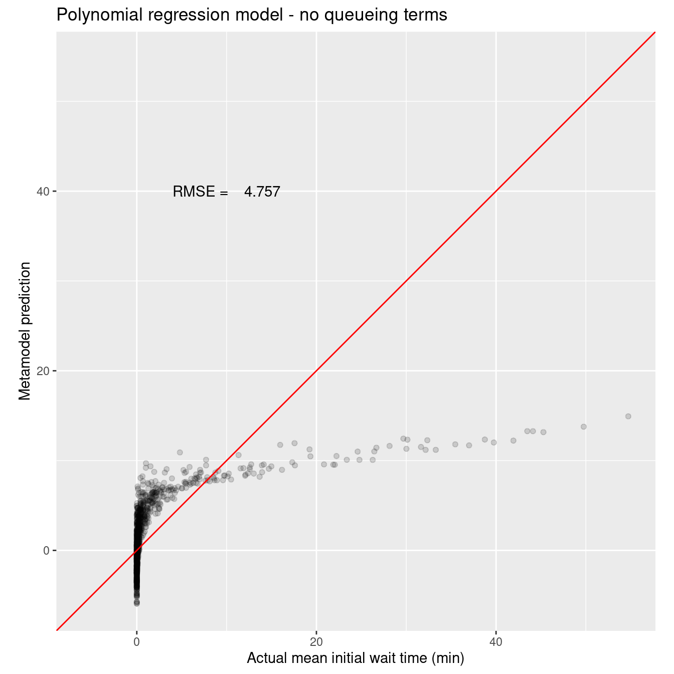

Not great, pretty horrible. Clearly some wierdness with the zero values of actual mean wait time. Let’s see how the addition of the queuing inspired features affects model accuracy. We’ll pull everything we did above into a single code chunk.

# Create a formula object. 
wait_i_poly_q_formula <- mean_wait_i ~ patients_per_clinic_block + 
                         num_med_techs +
                         num_rooms + 
                         vitals_time_mean +
                         exam_time_mean +
                         exam_time_cv2 + 
                         post_exam_time_mean +
                         off_util_staff + off_util_physician + off_util_room +
                         mean_wait_i_dm1

# Create recipe
wait_i_poly_q_recipe <- recipe(wait_i_poly_q_formula, data = xy_q_in_train) %>% 
  step_poly(patients_per_clinic_block, num_med_techs, num_rooms,
          vitals_time_mean, exam_time_mean, exam_time_cv2, post_exam_time_mean,
          off_util_staff, off_util_physician, off_util_room, mean_wait_i_dm1,
          degree = 2)

# Create workflow object (uses model object we created earlier)
wait_i_poly_q_wflow <- 
  workflow() %>% 
  add_model(wait_i_poly_mod) %>% 
  add_recipe(wait_i_poly_q_recipe)

# Fit the models
keep_pred <- control_resamples(save_pred = TRUE, save_workflow = FALSE)

wait_i_poly_q_results <- 
  wait_i_poly_q_wflow %>% 
  fit_resamples(resamples = in_train_splits, control = keep_pred)

collect_metrics(wait_i_poly_q_results)

# A tibble: 2 × 6
  .metric .estimator  mean     n std_err .config             
  <chr>   <chr>      <dbl> <int>   <dbl> <chr>               
1 rmse    standard   1.82     50 0.0219  Preprocessor1_Model1
2 rsq     standard   0.916    50 0.00266 Preprocessor1_Model1

# Do last fit
wait_i_last_poly_q_results <- last_fit(wait_i_poly_q_wflow, xy_q_in_split)

collect_metrics(wait_i_last_poly_q_results)

# A tibble: 2 × 4
  .metric .estimator .estimate .config             
  <chr>   <chr>          <dbl> <chr>               
1 rmse    standard       1.76  Preprocessor1_Model1
2 rsq     standard       0.917 Preprocessor1_Model1

wait_i_last_poly_q_rmse <- collect_metrics(wait_i_last_poly_q_results) %>% 
  filter(.metric == 'rmse') %>% 
  pull(.estimate) 

# Grab the predictions on the test data
assess_wait_i_last_poly_q_results <- collect_predictions(wait_i_last_poly_q_results)

# Plot actual vs predicted.
assess_wait_i_last_poly_q_results %>% 
  ggplot(aes(x = mean_wait_i, y = .pred)) + 
  geom_point(alpha = .15) +
  geom_abline(color = "red") + 
  coord_obs_pred() + 
  xlab("Actual mean initial wait time (min)") +
  ylab("Metamodel prediction") +
  ggtitle("Polynomial regression model - including queueing terms") +
  annotate("text", x = 10, y = 40, label = sprintf("RMSE = %8.3f", wait_i_last_poly_q_rmse))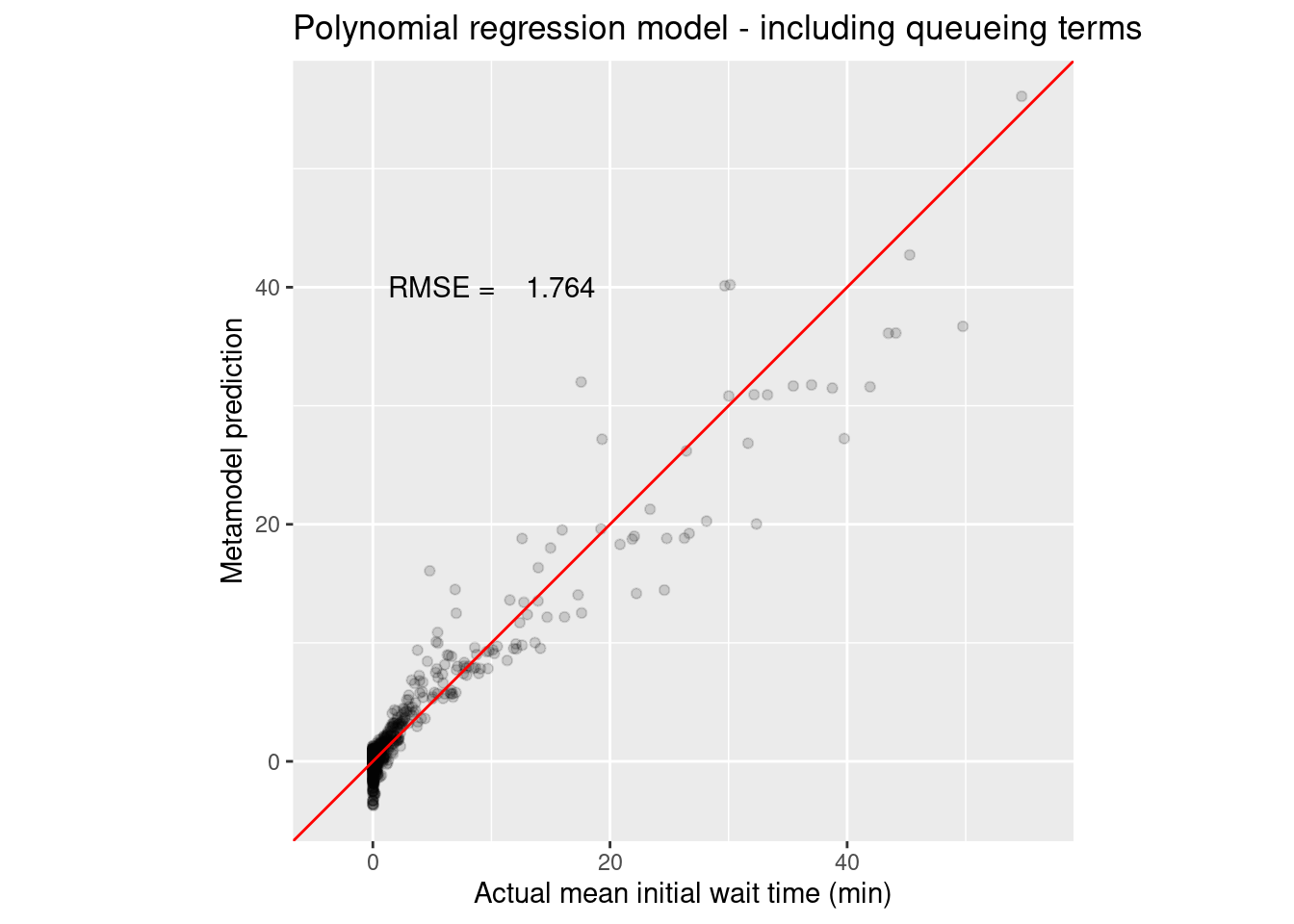

Clearly there is value in the queueing inspired terms. Ok, that’s the polynomial regression model. Tidymodels made it easy to create a coherent workflow that was easy to modify. For example, we could use step_ns instead of step_poly in the recipe and we could fit a natural cubic spline.

Now let’s look at the more complicated case of using tidymodels to fit a nonlinear model with nls().

Nonlinear queueing inspired model for initital wait

In the dataset, you’ll find a queueing related featured named mean_wait_i_dm1 which corresponds to a \(D/M/1\) based approximation for the initial mean wait time. The details are available in our paper, but for now we’ll just say that we fit a multiplicative power model that includes terms that attempt to correct for the violated assumptions of the \(D/M/1\) model.

The proposed model is

\[ W_I = b_1 \frac{W_{D}^{b_2}R^{b_3}C^{b_4}}{S^{b_5}} \]

where

\(W_{D}\) is the mean wait in the approximating \(D/M/1\) queue
\(R\) is the number of exam rooms
\(C\) is the coefficient of variation squared of an approximate effective service time distribution for staff (hyper-erlang)
\(S\) is the number medical technician staff

You can think of the \(R, C, S\) terms along with the power parameters as being adjustments to the raw \(D/M/1\) based term, \(W_{D}\). Clearly, this is a nonlinear model and we will estimate \(b_1, ..., b_5\) using R’s nls() function.

Developing a parsnip model that uses nls()

It would be great if we could simply use similar code to what we did above for the polynomial models. Unfortunately, it’s not that easy. To begin with, nonlinear regression, and in particular the nls() engine isn’t supported as of yet in parsnip, the tidymodels package that handles model building. As I starting digging into (no pun intended) this package for the first time, I realized, of course, a “parsnip” is not a “carrot”. The goal of parsnip, written by the same author who developed the caret package, is stated on their webpage.

The goal of parsnip is to provide a tidy, unified interface to models that can be used to try a range of models without getting bogged down in the syntactical minutiae of the underlying packages.

However, parsnip is not the new caret. It’s more like tidymodels is the new caret. Parsnip just handles the unified modeling interface and has been designed with the goal of being easy for users to add their own custom models. They have a very nice tutorial on doing just that:

How to build a parsnip model

So, let’s create our own "nonlinear_reg" model that relies on nls() as the model fitting engine. Since nls() needs a starting guess for the parameter values, we need to figure out how and where such a starting guess fits into a custom parsnip model.

I just followed the steps in the tutorial listed above.

Step 1. Register the model, modes, and arguments

set_new_model("nonlinear_reg")
set_model_mode(model = "nonlinear_reg", mode = "regression")
set_model_engine(
  "nonlinear_reg", 
  mode = "regression", 
  eng = "nls"
)
set_dependency("nonlinear_reg", eng = "nls", pkg = "stats")

# We can examine what we just created
show_model_info("nonlinear_reg")

Information for `nonlinear_reg`
 modes: unknown, regression 

 engines: 
   regression: nlsNA

¹The model can use case weights.

 no registered arguments.

 no registered fit modules.

 no registered prediction modules.

Step 2. Create the model function

Now we declare the main arguments for the model. This is intended for tuning parameters (I think) and isn’t needed here.

# set_model_arg(
#   model = "nonlinear_reg",
#   eng = "nls",
#   parsnip = "start",
#   original = "start",
#   # Not sure what to use for func arg
#   func = list(pkg = "foo", fun = "bar"),
#   has_submodel = FALSE
# )
# show_model_info("nonlinear_reg")

This next function creates the new_model_spec object needed to define our custom model.

nonlinear_reg <-
  function(mode = "regression",  start = NULL) {
    # Check for correct mode
    if (mode  != "regression") {
      rlang::abort("`mode` should be 'regression'")
    }
    
    # Capture the arguments in quosures
    args <- list(start = rlang::enquo(start))
    
    # Create specification
    new_model_spec(
      "nonlinear_reg",
      args = args,
      mode = mode,
      engine = NULL,
      eng_args = NULL,
      method = NULL
    )
  }

Step 3. Add a fit module

set_fit(
  model = "nonlinear_reg",
  eng = "nls",
  mode = "regression",
  value = list(
    interface = "formula",
    protect = c("formula", "data"),
    func = c(pkg = "stats", fun = "nls"),
    defaults = list()
  )
)

show_model_info("nonlinear_reg")

Information for `nonlinear_reg`
 modes: unknown, regression 

 engines: 
   regression: nls

¹The model can use case weights.

 no registered arguments.

 fit modules:
 engine       mode
    nls regression

 no registered prediction modules.

set_encoding(
  model = "nonlinear_reg",
  eng = "nls",
  mode = "regression",
  options = list(
    predictor_indicators = "none",
    compute_intercept = FALSE,
    remove_intercept = FALSE,
    allow_sparse_x = FALSE
  )
)

Step 4. Add modules for prediction

response_info <- 
  list(
    pre = NULL,
    post = NULL,
    func = c(fun = "predict"),
    args =
      # These lists should be of the form:
      # {predict.nls argument name} = {values provided from parsnip objects}
      list(
        # We don't want the first two arguments evaluated right now
        # since they don't exist yet. 
        object = quote(object$fit),
        newdata = quote(new_data)
      )
  )

set_pred(
  model = "nonlinear_reg",
  eng = "nls",
  mode = "regression",
  type = "numeric",
  value = response_info
)

Now we have a custom model type named nonlinear_reg that we can use just like (we hope) any built in parsnip model. Before trying to use with the full blown resampling scheme, let’s just see if we can make it work for a simple fit, predict, and assess cycle. We’ll just fit the model on the entire within design training set, xy_q_in_train.

The nls() function would like a vector of initial values for all parameters to be fit.

init_nls_wait_i <- c(b1=.1, b2=-0.6, b3=2, b4=0.5, b5=2)

Create a model object, a formula object and then fit the model.

# Create nonlinear_reg model object
wait_i_nls_mod <- nonlinear_reg() %>% set_engine(engine = "nls", start = init_nls_wait_i)

# Create the nonlinear formula
wait_i_nls_mod_formula <- mean_wait_i ~ b1 * (num_med_techs ^ b2) * 
  (mean_wait_i_dm1 ^ b3) *(num_rooms ^ b4) * (staff_eff_svc_time_cv2 ^ b5)

# Fit the model
wait_i_nls_fit <- wait_i_nls_mod %>% 
  fit(formula = wait_i_nls_mod_formula, data = xy_q_in_train)

wait_i_nls_fit

parsnip model object

Nonlinear regression model
  model: mean_wait_i ~ b1 * (num_med_techs^b2) * (mean_wait_i_dm1^b3) *     (num_rooms^b4) * (staff_eff_svc_time_cv2^b5)
   data: data
      b1       b2       b3       b4       b5 
 0.01395 -0.33003  1.64832  0.54281  0.38448 
 residual sum-of-squares: 4656

Number of iterations to convergence: 7 
Achieved convergence tolerance: 1.525e-06

Great. It works. We can make predictions and compute error metrics.

wait_i_nls_predicted <- predict(wait_i_nls_fit, new_data = xy_q_in_test)

wait_i_nls_rmse <- rmse_vec(xy_q_in_test$mean_wait_i, wait_i_nls_predicted$.pred)

# Plot actual vs predicted.
xy_q_in_test %>% 
  select(mean_wait_i) %>% 
  bind_cols(wait_i_nls_predicted) %>%  
  ggplot(aes(x = mean_wait_i, y = .pred)) + 
  geom_point(alpha = .15) +
  geom_abline(color = "red") + 
  coord_obs_pred() + 
  xlab("Actual mean initial wait time (min)") +
  ylab("Metamodel prediction") +
  ggtitle("Nonlinear queueing based model") +
  annotate("text", x = 10, y = 40, label = sprintf("RMSE = %8.3f", wait_i_nls_rmse))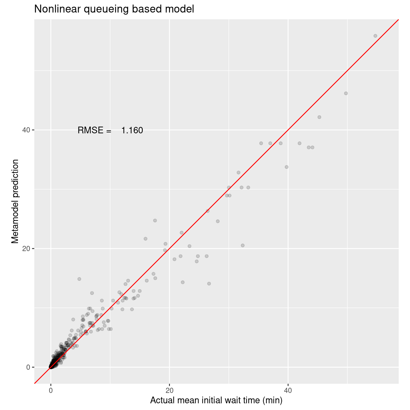

Very nice fit and only five parameters that have physical underpinnings that make sense in the context of queueing models.

To get a sense of the stability of the model, We really need to add the k-crossfold resampling just as we did with the polynomial models. Before we try that, we can actually get a preview of the impending problem by tweaking the previous example to use a simple tidy workflow object. The model and formula objects are fine. Let’s try to use them use them in a workflow.

# Create simple workflow
wait_i_nls_wf <- workflow() %>% 
  add_model(wait_i_nls_mod) %>% 
  add_formula(wait_i_nls_mod_formula)

# Pipe the workflow into fit() to fit the model
wait_i_nls_wf %>% 
  fit(data = xy_q_in_train)

Error in terms.formula(formula, data = data): invalid power in formula

And there’s the problem. When workflows::add_formula is called, an internal checking of the proposed formula flags our formula as having an invalid power. No doubt this is because the powers in our formula are parameters to be estimated by nls(). This same problem also occurs if we try to use fit_resample as we did with the polynomial models.

To summarize what we just learned, While I was able to successfully use my custom nonlinear_reg model to fit a model and assess its predictive accuracy, I cannot use it in any workflow that uses add_formula or fit_resamples() So, it appears that we are going to have to write our own function for iterating over our k-crossfold splits object and fitting and assessing models for each split.

Fit queueing based nls model and use cross-validation

I hacked together a few functions to do what tune::fit_resamples() does. They basically just loop through the splits doing model fitting, predicting, scoring and plotting. You can find the source code here within the GitHub repo for this project.

source('lib/myparsnip_funcs.R')

# Create nonlinear_reg model object
init_nls_wait_i <- c(b1=.1, b2=-0.6, b3=2, b4=0.5, b5=2)
wait_i_nls_mod <- nonlinear_reg() %>% set_engine(engine = "nls", start = init_nls_wait_i)

# Create the nonlinear formula
wait_i_nls_mod_formula <- mean_wait_i ~ b1 * (num_med_techs ^ b2) * 
  (mean_wait_i_dm1 ^ b3) *(num_rooms ^ b4) * (staff_eff_svc_time_cv2 ^ b5)

# Call my custom function to fit the models for each split
wait_i_kfold_res <- myparsnip_fit_resamples(wait_i_nls_mod, wait_i_nls_mod_formula,
                                          in_train_splits, kfold_number, kfold_repeats)

Warning: `aes_string()` was deprecated in ggplot2 3.0.0.
ℹ Please use tidy evaluation ideoms with `aes()`

Now let’s look at the metrics averaged over the 50 splits (10 repeats x 5 folds). The standard error is small and the RMSE value for this nonlinear model is better than both the spline and poly RMSE values. While I attempted to have myparsnip_fit_resamples() return an object that I could pass directly to tune::collect_metrics, I couldn’t quite get it to work even after digging into the source code and finding that tune::collect_metrics calls UseMethod and trying to coerce my function return value to be of the correct class so that the correct method would get dispatched. Then I realized I could just call the desired method even though it doesn’t get exported into the namespace for tune by using the triple colon notation.

tune:::collect_metrics.tune_results(wait_i_kfold_res, summarize = TRUE)

# A tibble: 2 × 6
  .metric .estimator  mean     n std_err .config             
  <chr>   <chr>      <dbl> <int>   <dbl> <chr>               
1 mae     standard   0.472    50 0.00548 Preprocessor1_Model1
2 rmse    standard   1.29     50 0.0189  Preprocessor1_Model1

Now we’ll refit one last model using the entire training set and assess its performance on the in design test data - again using a custom function.

# Do last fit
wait_i_last_res <- myparsnip_last_fit(wait_i_nls_mod, wait_i_nls_mod_formula, xy_q_in_split)

tune:::collect_metrics.tune_results(wait_i_last_res$metrics_summary, summarize = FALSE)

# A tibble: 2 × 5
  id        .metric .estimator .estimate .config             
  <chr>     <chr>   <chr>          <dbl> <chr>               
1 Resample1 rmse    standard       1.16  Preprocessor1_Model1
2 Resample1 mae     standard       0.418 Preprocessor1_Model1

No we can check out the actual vs predicted plot based on the test data. This plot also shows that the queueing based model outperforms the polynomial regression models - and only has 5 parameters whereas the polynomial models have many parameters (10 base inputs plus 10 quadratic terms). As an aside, a natural cubic spline model with one knot performed very similarly to the polynomial regression model.

wait_i_last_res$act_vs_pred_plot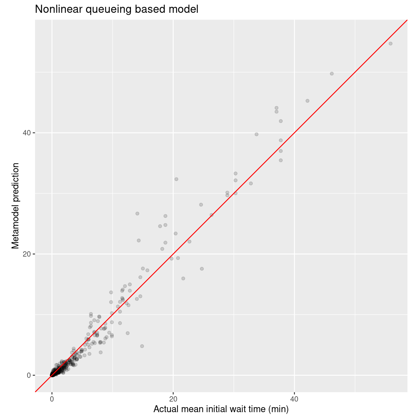

Random forest model

Just for grins, let’s try a totally different type of model - a random forest. Again, we’ll create one model without the queueing related terms and one with. Tidymodels makes it easy to reuse code - just drop in a different model engine.

wait_i_rf_mod <- rand_forest(mode = "regression") %>% 
  set_engine(engine = "ranger")

# Create a formula object. 
wait_i_rf_q_formula <- mean_wait_i ~ patients_per_clinic_block + 
                         num_med_techs +
                         num_rooms + 
                         vitals_time_mean +
                         exam_time_mean +
                         exam_time_cv2 + 
                         post_exam_time_mean +
                         off_util_staff + off_util_physician + off_util_room +
                         mean_wait_i_dm1

# Create recipe
wait_i_rf_q_recipe <- recipe(wait_i_rf_q_formula, data = xy_q_in_train) %>% 
  step_poly(patients_per_clinic_block, num_med_techs, num_rooms,
          vitals_time_mean, exam_time_mean, exam_time_cv2, post_exam_time_mean,
          off_util_staff, off_util_physician, off_util_room, mean_wait_i_dm1,
          degree = 2)

# Create workflow object (uses model object we created earlier)
wait_i_rf_q_wflow <- 
  workflow() %>% 
  add_model(wait_i_rf_mod) %>% 
  add_recipe(wait_i_rf_q_recipe)

# Fit the models
keep_pred <- control_resamples(save_pred = TRUE, save_workflow = FALSE)

wait_i_rf_q_results <- 
  wait_i_rf_q_wflow %>% 
  fit_resamples(resamples = in_train_splits, control = keep_pred)

collect_metrics(wait_i_rf_q_results)

# A tibble: 2 × 6
  .metric .estimator  mean     n  std_err .config             
  <chr>   <chr>      <dbl> <int>    <dbl> <chr>               
1 rmse    standard   0.765    50 0.0221   Preprocessor1_Model1
2 rsq     standard   0.986    50 0.000678 Preprocessor1_Model1

# Do last fit
wait_i_last_rf_q_results <- last_fit(wait_i_rf_q_wflow, xy_q_in_split)

collect_metrics(wait_i_last_rf_q_results)

# A tibble: 2 × 4
  .metric .estimator .estimate .config             
  <chr>   <chr>          <dbl> <chr>               
1 rmse    standard       0.586 Preprocessor1_Model1
2 rsq     standard       0.991 Preprocessor1_Model1

wait_i_last_rf_q_rmse <- collect_metrics(wait_i_last_rf_q_results) %>% 
  filter(.metric == 'rmse') %>% 
  pull(.estimate) 

# Grab the predictions on the test data
assess_wait_i_last_rf_q_results <- collect_predictions(wait_i_last_rf_q_results)

# Plot actual vs predicted.
assess_wait_i_last_rf_q_results %>% 
  ggplot(aes(x = mean_wait_i, y = .pred)) + 
  geom_point(alpha = .15) +
  geom_abline(color = "red") + 
  coord_obs_pred() + 
  xlab("Actual mean initial wait time (min)") +
  ylab("Metamodel prediction") +
  ggtitle("Random forest model - including queueing terms") +
  annotate("text", x = 10, y = 40, label = sprintf("RMSE = %8.3f", wait_i_last_rf_q_rmse))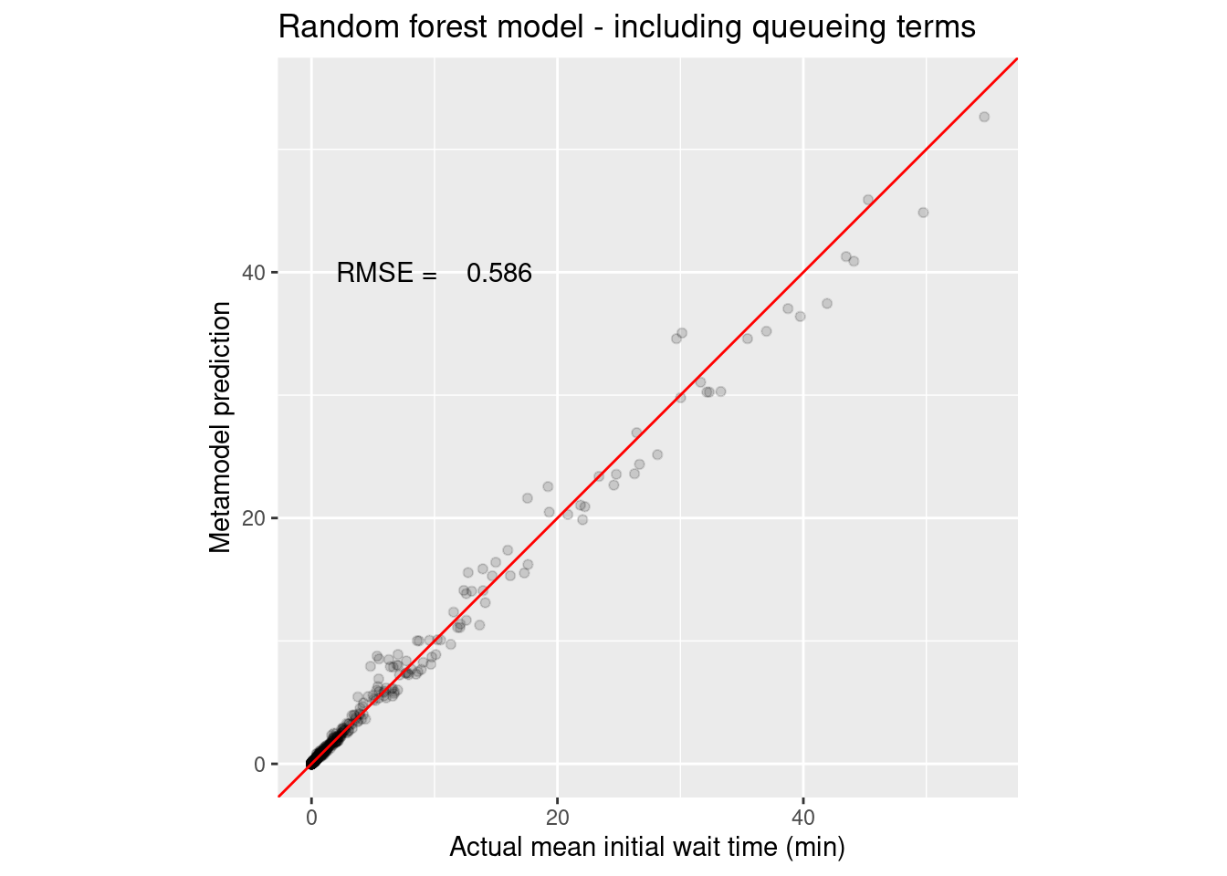

Wow, those random forests can be tough to beat. Let’s see if the queueing related features helped the random forest by dropping those four terms from the formula.

wait_i_rf_mod <- rand_forest(mode = "regression") %>% 
  set_engine(engine = "ranger")

# Create a formula object. 
wait_i_rf_noq_formula <- mean_wait_i ~ patients_per_clinic_block + 
                         num_med_techs +
                         num_rooms + 
                         vitals_time_mean +
                         exam_time_mean +
                         exam_time_cv2 + 
                         post_exam_time_mean

# Create recipe
wait_i_rf_noq_recipe <- recipe(wait_i_rf_noq_formula, data = xy_q_in_train) %>% 
  step_poly(patients_per_clinic_block, num_med_techs, num_rooms,
          vitals_time_mean, exam_time_mean, exam_time_cv2, post_exam_time_mean,
          degree = 2)

# Create workflow object (uses model object we created earlier)
wait_i_rf_noq_wflow <- 
  workflow() %>% 
  add_model(wait_i_rf_mod) %>% 
  add_recipe(wait_i_rf_noq_recipe)

# Fit the models
keep_pred <- control_resamples(save_pred = TRUE, save_workflow = FALSE)

wait_i_rf_noq_results <- 
  wait_i_rf_noq_wflow %>% 
  fit_resamples(resamples = in_train_splits, control = keep_pred)

collect_metrics(wait_i_rf_noq_results)

# A tibble: 2 × 6
  .metric .estimator  mean     n std_err .config             
  <chr>   <chr>      <dbl> <int>   <dbl> <chr>               
1 rmse    standard   1.71     50 0.0393  Preprocessor1_Model1
2 rsq     standard   0.951    50 0.00167 Preprocessor1_Model1

# Do last fit
wait_i_last_rf_noq_results <- last_fit(wait_i_rf_noq_wflow, xy_q_in_split)

collect_metrics(wait_i_last_rf_noq_results)

# A tibble: 2 × 4
  .metric .estimator .estimate .config             
  <chr>   <chr>          <dbl> <chr>               
1 rmse    standard       1.57  Preprocessor1_Model1
2 rsq     standard       0.963 Preprocessor1_Model1

wait_i_last_rf_noq_rmse <- collect_metrics(wait_i_last_rf_noq_results) %>% 
  filter(.metric == 'rmse') %>% 
  pull(.estimate) 

# Grab the predictions on the test data
assess_wait_i_last_rf_noq_results <- collect_predictions(wait_i_last_rf_noq_results)

# Plot actual vs predicted.
assess_wait_i_last_rf_noq_results %>% 
  ggplot(aes(x = mean_wait_i, y = .pred)) + 
  geom_point(alpha = .15) +
  geom_abline(color = "red") + 
  coord_obs_pred() + 
  xlab("Actual mean initial wait time (min)") +
  ylab("Metamodel prediction") +
  ggtitle("Random forest model - no queueing terms") +
  annotate("text", x = 10, y = 40, label = sprintf("RMSE = %8.3f", wait_i_last_rf_noq_rmse))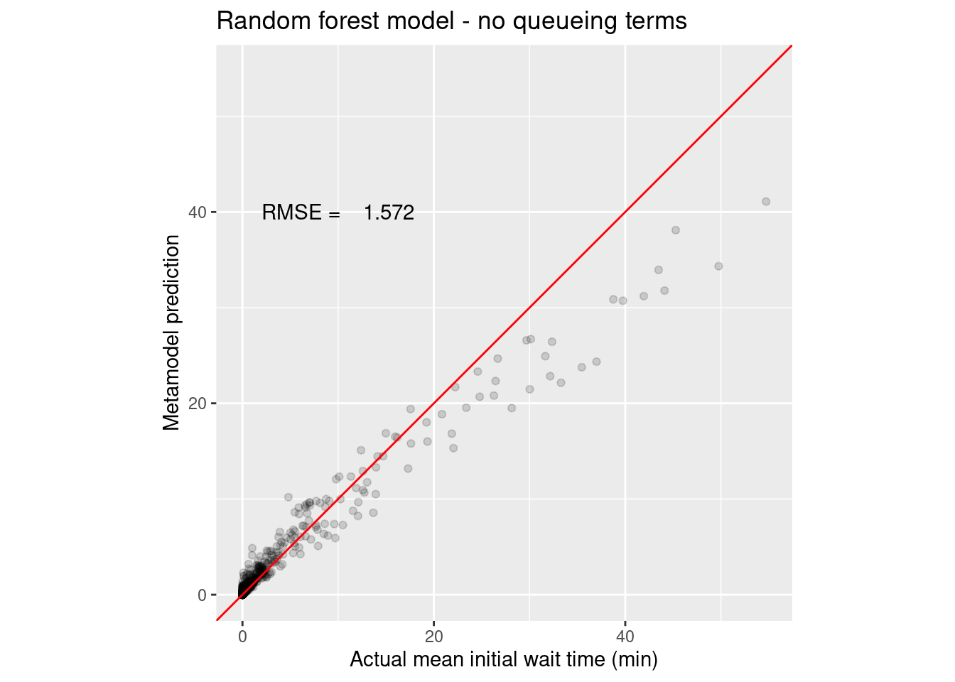

Yep, the queueing terms definitely helped with the random forest as they did with the polynomial regression model. You can see how there is systematic under prediction for larger wait times.

Out of design analysis

Now let’s compare the models on their ability to extrapolate beyond the experimental design points. All of the models contain the queueing inspired features. Start with the polynomial model.

wait_i_poly_out_q_wflow <- 
  workflow() %>% 
  add_model(wait_i_poly_mod) %>% 
  add_recipe(wait_i_poly_q_recipe)
  
wait_i_poly_out_fit_q <- fit(wait_i_poly_out_q_wflow, data = xy_q_in)
wait_i_poly_out_pred_q <- predict(wait_i_poly_out_fit_q, new_data = xy_q_out)


# Plot actual vs predicted.
xy_q_out %>% 
  select(mean_wait_i) %>% 
  bind_cols(wait_i_poly_out_pred_q) %>%  
  ggplot(aes(x = mean_wait_i, y = .pred)) + 
  geom_point(alpha = .15) +
  geom_abline(color = "red") + 
  coord_obs_pred() + 
  xlab("Actual mean initial wait time (min)") +
  ylab("Metamodel prediction") +
  ggtitle("Polynomial model - out of design extrapolation")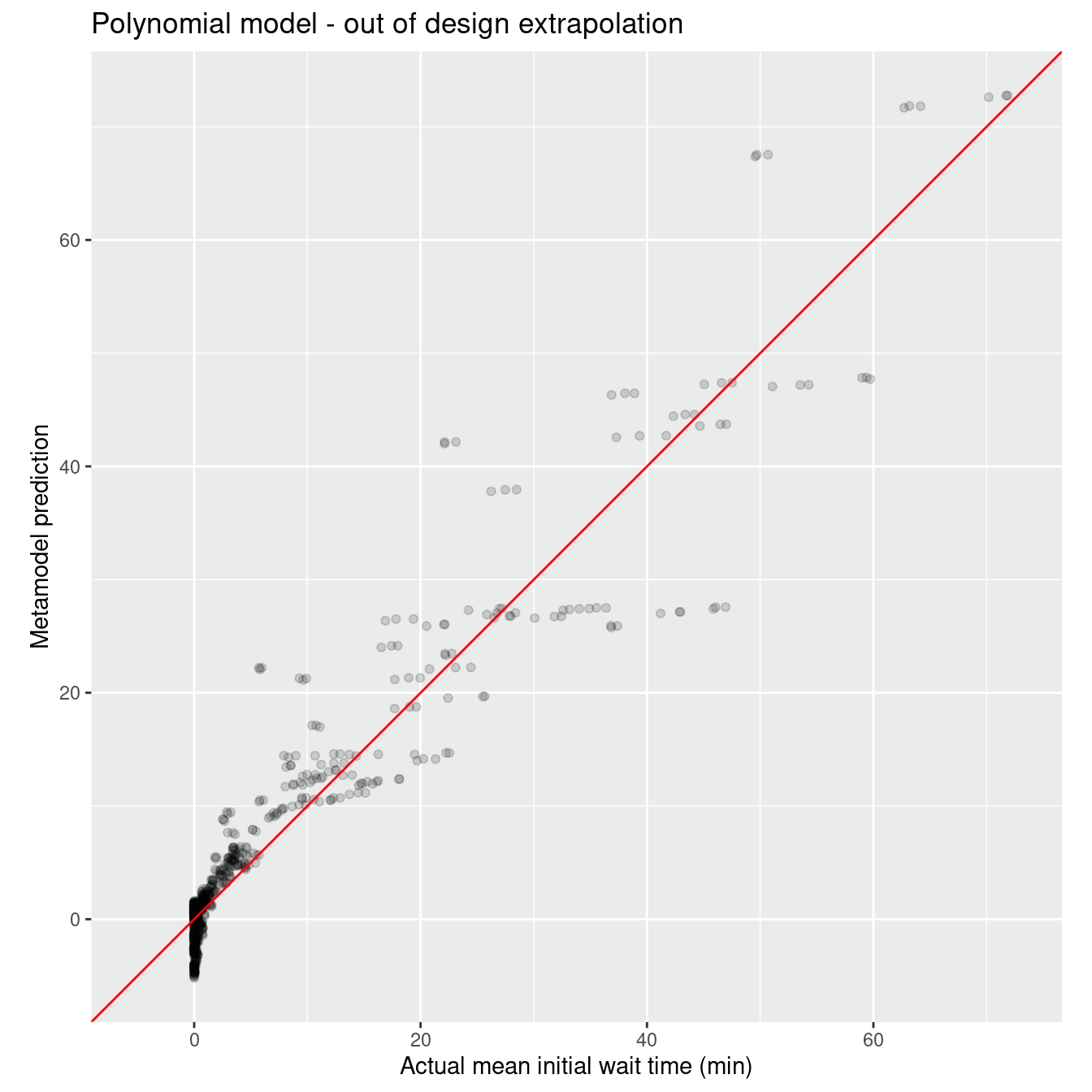

wait_i_poly_out_rmse_q <- rmse_vec(xy_q_out$mean_wait_i, wait_i_poly_out_pred_q$.pred)

sprintf("RMSE for poly model on out of design points: %10.3f", wait_i_poly_out_rmse_q)

[1] "RMSE for poly model on out of design points:      3.408"

Now for the random forest.

wait_i_rf_out_wflow_q <- 
  workflow() %>% 
  add_model(wait_i_rf_mod) %>% 
  add_recipe(wait_i_rf_q_recipe)

wait_i_rf_out_wflow_noq <- 
  workflow() %>% 
  add_model(wait_i_rf_mod) %>% 
  add_recipe(wait_i_rf_noq_recipe)

wait_i_rf_out_fit_q <- fit(wait_i_rf_out_wflow_q, data = xy_q_in)
wait_i_rf_out_pred_q <- predict(wait_i_rf_out_fit_q, new_data = xy_q_out)

wait_i_rf_out_fit_noq <- fit(wait_i_rf_out_wflow_noq, data = xy_q_in)
wait_i_rf_out_pred_noq <- predict(wait_i_rf_out_fit_noq, new_data = xy_q_out)

# Plot actual vs predicted.
xy_q_out %>% 
  select(mean_wait_i) %>% 
  bind_cols(wait_i_rf_out_pred_q) %>%  
  ggplot(aes(x = mean_wait_i, y = .pred)) + 
  geom_point(alpha = .15) +
  geom_abline(color = "red") + 
  coord_obs_pred() + 
  xlab("Actual mean initial wait time (min)") +
  ylab("Metamodel prediction") +
  ggtitle("Random forest model - out of design extrapolation")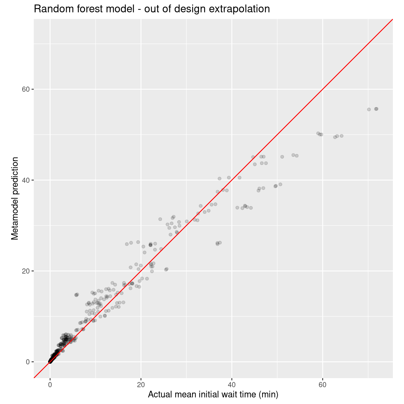

wait_i_rf_out_rmse_q <- rmse_vec(xy_q_out$mean_wait_i, wait_i_rf_out_pred_q$.pred)
wait_i_rf_out_rmse_noq <- rmse_vec(xy_q_out$mean_wait_i, wait_i_rf_out_pred_noq$.pred)

sprintf("RMSE for rf model on out of design points with queueing: %10.3f", wait_i_rf_out_rmse_q)

[1] "RMSE for rf model on out of design points with queueing:      2.195"

sprintf("RMSE for rf model on out of design points, no queueing: %10.3f", wait_i_rf_out_rmse_noq)

[1] "RMSE for rf model on out of design points, no queueing:      3.889"

Finally, here’s the nonlinear model.

# Nonlinear models need starting guesses for the params
init_nls_wait_i <- c(b1=.1, b2=-0.6, b3=2, b4=0.5, b5=2)

# Fit the model
wait_i_nls_out_fit <- nls(mean_wait_i ~ b1 * (num_med_techs ^ b2) * 
  (mean_wait_i_dm1 ^ b3) *(num_rooms ^ b4) * (staff_eff_svc_time_cv2 ^ b5),
                 data=xy_q_in, start=init_nls_wait_i)

wait_i_nls_out_pred <- predict(wait_i_nls_out_fit, newdata = xy_q_out)
#wait_i_nls_out_pred <- enframe(wait_i_nls_out_pred, name=NULL, value="wait_i_nls_out_pred")

wait_i_nls_out_rmse <- rmse_vec(xy_q_out$mean_wait_i, wait_i_nls_out_pred)
sprintf("RMSE for nls model on out of design points: %10.3f", wait_i_nls_out_rmse)

[1] "RMSE for nls model on out of design points:      3.033"

nls_plot_data <- xy_q_out %>%
  select(mean_wait_i) %>%
  bind_cols(wait_i_nls_out_pred)

New names:
• `` -> `...2`

ggplot(data=nls_plot_data, aes(x = mean_wait_i, y = wait_i_nls_out_pred)) +
  geom_point(alpha = .15) +
  geom_abline(color = "red") +
  coord_obs_pred() +
  xlab("Actual mean initial wait time (min)") +
  ylab("Metamodel prediction") +
  ggtitle("Queueing based model - out of design extrapolation")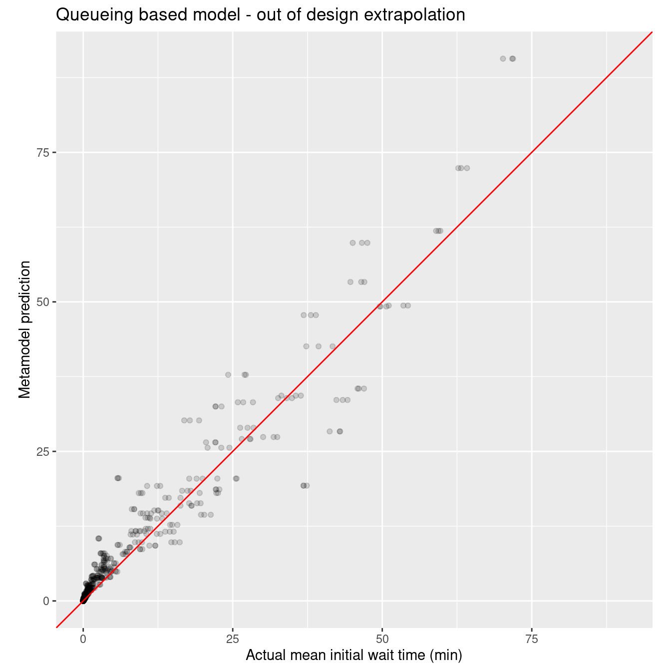

Like I said earlier, those darn random forests are tough to beat. :)

Key takeaways

The bottom line is that:

we used a queueing inspired nonlinear model with only five parameters that outperformed polynomial and spline models with many more parameters in both in and out of design predictions (interpolation and extrapolation). The random forest model outperformed all three other techniques on the in design dataset but exhibited some systematic bias on the out of design dataset. Of course, the random forest model is a black box in comparison to the regression models.
the nonlinear queueing based model made sense in the context of the underlying process physics of the simulation model - each term was interpretable and had basis in theory,
there is no simple cookbook procedure to exploiting domain knowledge (queueing knowledge in this case). Each situation is different and the details of the feature engineering are going to be situational. It’s unrealistic to expect more.
offered load and resource utilization based features are often simple to develop and can be quite predictive.

Citation

BibTeX citation:

@online{isken2023,
  author = {Mark Isken},
  title = {Using Tidymodels for Simulation Metamodeling},
  date = {2023-02-12},
  langid = {en}
}

For attribution, please cite this work as:

Mark Isken. 2023. “Using Tidymodels for Simulation Metamodeling.” February 12, 2023.