Comparing predictive models for obstetrical unit occupancy using caret - Part 1
Fitting predictive metamodels
Simulation metamodeling involves building predictive models based on outputs of designed simulation experiments. In this series of posts we’ll share our experience with using the R package caret for building and comparing several predictive modeling based metamodels including linear models, neural networks, random forests, k-nearest neighbor, and cubic splines.
Simulating hospital inpatient obstetrical units for capacity planning
A typical configuration of hospital units which provide care for women about to give birth might include an observation unit, a labor, delivery and recovery unit (LDR) and a postpartum (PP) unit. Matching the capacity of these units to demand placed on them is important for maintaining smooth patient flow. For example, there should be sufficient capacity in a PP unit so that there is a relatively small probability that a post-delivery patient is blocked in the LDR due to lack of a bed in PP. Of course, complicating the capacity planning process is the fact that there are numerous sources of uncertainty in obstetrical patient care processes. These include the number and timing of patient arrivals, whether or not the patient requires a C-section and the length of stay in each of the three units.

I’m working on a research project involving capacity planning models for these systems. One phase involves building what are known as simulation metamodels. The main components are:
- built a discrete event simulation model of a simplified queueing network model of typical obstetrical patient flow system.
- designed and ran a set of simulation experiments involving a range patient volumes, percentages of patients requiring c-section, and unit sizes (numbers of beds). There were 150 scenarios simulated.
- post-processed the output using both R and Python to compute several performance measures related to unit occupancy and patient delays.
- now working on building and comparing a number of different statistical/machine learning techniques for predicting occupancy and delay related peformance measures using the experimental inputs (volume, % c-section, unit sizes). This is where
caretcomes in.
In the simulation world, this last step is known as simulation metamodeling. It has a long history. See any good discrete event simulation text such as Simulation modeling and analysis by Law and Kelton for an overview. There’s also a nice overview done by R. Barton and available as a free pdf from the Proceedings of the 2015 Winter Simulation Conference. Typically, techniques s any predictive modeling technique capable of producing real valued output such as neural networks, regression trees, k-nearest neighbor or any number of advanced regression techniques. As this was my first significant project using caret, I thought it would be helpful to write up some of the challenges faced and share some of the techniques I used to make it easier to compare different models. In this first post we will use caret to train a few models, make predictions, summarize their performance and motivate the need for a way to automate this workflow to make it easier to compare a number of modeling techniques and associated meta-settings such as the relative size of the training and test datasets.
Read in the data.
As mentioned above, there are 150 scenarios (rows) and a number of input and output columns. For this series of posts, I’ve created an example file containing a limited number of the output related columns.
Let’s read in the data.
obsim_df <- read.csv(file="data/obsim_example.csv")
names(obsim_df)[1] <- "scenario"
# Shorten a few column names
names(obsim_df)[13] <- "occmean_ldr"
names(obsim_df)[14] <- "occp95_ldr"
names(obsim_df)[15] <- "occmean_pp"
names(obsim_df)[16] <- "occp95_pp"
Here are the input variables and the first few rows:
knitr::kable(head(obsim_df[,2:12]),digits=2)| lam_ldr | alos_ldr | cap_ldr | load_ldr | rho_ldr | lam_pp | alos_pp | cap_pp | load_pp | rho_pp | tot_c_rate |
|---|---|---|---|---|---|---|---|---|---|---|
| 2.74 | 0.5 | 4 | 1.37 | 0.34 | 2.74 | 2.2 | 12 | 6.03 | 0.50 | 0.2 |
| 2.74 | 0.5 | 4 | 1.37 | 0.34 | 2.74 | 2.2 | 10 | 6.03 | 0.60 | 0.2 |
| 2.74 | 0.5 | 4 | 1.37 | 0.34 | 2.74 | 2.2 | 9 | 6.03 | 0.67 | 0.2 |
| 2.74 | 0.5 | 3 | 1.37 | 0.46 | 2.74 | 2.2 | 12 | 6.03 | 0.50 | 0.2 |
| 2.74 | 0.5 | 3 | 1.37 | 0.46 | 2.74 | 2.2 | 10 | 6.03 | 0.60 | 0.2 |
| 2.74 | 0.5 | 3 | 1.37 | 0.46 | 2.74 | 2.2 | 9 | 6.03 | 0.67 | 0.2 |
… and the output variables
knitr::kable(head(obsim_df[,13:16]), digits=3)| occmean_ldr | occp95_ldr | occmean_pp | occp95_pp |
|---|---|---|---|
| 1.371 | 3.680 | 6.051 | 10.183 |
| 1.426 | 3.987 | 6.017 | 10.000 |
| 1.518 | 4.000 | 6.020 | 9.000 |
| 1.319 | 3.000 | 6.021 | 10.231 |
| 1.362 | 3.000 | 6.031 | 10.000 |
| 1.431 | 3.000 | 6.033 | 9.000 |
str(obsim_df)## 'data.frame': 150 obs. of 16 variables:
## $ scenario : int 1 2 3 4 5 6 7 8 9 10 ...
## $ lam_ldr : num 2.74 2.74 2.74 2.74 2.74 ...
## $ alos_ldr : num 0.5 0.5 0.5 0.5 0.5 0.5 0.5 0.5 0.5 0.5 ...
## $ cap_ldr : int 4 4 4 3 3 3 2 2 2 8 ...
## $ load_ldr : num 1.37 1.37 1.37 1.37 1.37 ...
## $ rho_ldr : num 0.342 0.342 0.342 0.457 0.457 ...
## $ lam_pp : num 2.74 2.74 2.74 2.74 2.74 ...
## $ alos_pp : num 2.2 2.2 2.2 2.2 2.2 2.2 2.2 2.2 2.2 2.2 ...
## $ cap_pp : int 12 10 9 12 10 9 12 10 9 29 ...
## $ load_pp : num 6.03 6.03 6.03 6.03 6.03 ...
## $ rho_pp : num 0.502 0.603 0.67 0.502 0.603 ...
## $ tot_c_rate : num 0.2 0.2 0.2 0.2 0.2 0.2 0.2 0.2 0.2 0.2 ...
## $ occmean_ldr: num 1.37 1.43 1.52 1.32 1.36 ...
## $ occp95_ldr : num 3.68 3.99 4 3 3 ...
## $ occmean_pp : num 6.05 6.02 6.02 6.02 6.03 ...
## $ occp95_pp : num 10.2 10 9 10.2 10 ...Input Variables
| Name | Math | Description |
|---|---|---|
lam_ldr |
\(\lambda_L\) | Arrival rate of patients to LDR unit |
alos_ldr |
\(B_L\) | Average length of stay in LDR |
cap_ldr |
\(c_L\) | Number of beds in LDR |
load_ldr |
\(\lambda_L B_L\) | Arrival rate times average length of stay; a measure of workload submitted to the LDR |
rho_ldr |
\(\rho_L=\lambda_L B_L/c_L\) | Traffic intensity; a measure of congestion of LDR |
lam_pp |
\(\lambda_P\) | Arrival rate of patients to postpartum (PP) unit |
alos_pp |
\(B_P\) | Average length of stay in PP |
cap_pp |
\(c_P\) | Number of beds in PP |
load_pp |
\(\lambda_P B_P\) | Arrival rate times average length of stay; a measure of workload submitted to the PP |
rho_pp |
\(\rho_P=\lambda_P B_P/c_P\) | Traffic intensity; a measure of congestion of PP |
tot_c_rate |
\(\gamma\) | Percentage of patients requiring c-section |
Response Variables
| Name | Description |
|---|---|
occmean_ldr |
Mean occupancy (number of patients) in LDR unit |
occp95_ldr |
95th percentile of occupancy (number of patients) in LDR unit |
occmean_pp |
Mean occupancy (number of patients) in PP unit |
occp95_pp |
95th percentile of occupancy (number of patients) in PP unit |
There are other important response variables such as the probability that a patient gets blocked in the LDR due to the PP unit being full and the amount of time (mean, percentiles) that such blocked patients wait for a PP bed to become available. We’ll explore those variables in subsequent posts. For now, we’ll just focus on the mean and 95th percentile of occupancy in the LDR and PP units.
Metamodel 1 - Mean occupancy of PP
This is the simplest case since the PP unit behaves like an \(M/G/c\) queueing system for which mean occupancy is simply the load placed on the unit, \(\lambda_P B_P\). While the details of the simulation model are outside the scope of this first post, we will note that the length of stay in the PP unit is the mixture of two different distributions - one for patients requiring a c-section and one for those not requiring one. More on queueing models and simulation details in later posts.
It would seem that pretty much any technique such as a linear model, neural net, or random forest should be able to produce reasonable predictions. We’ll use this simple case to illustrate the basics of using the caret package to compare a few different models.
This isn’t meant to be a comprehensive tutorial on the basics of caret. There are plenty of those available and the documentation is a good place to start. Instead, we’ll use this simple example to motivate our desire to come up with a simple scheme for automating a bunch of caret runs for different models and values of experimental hyperparameters.
Load libraries
library(ggplot2)
library(Metrics) # Just to use its rmse() function
library(caret)
library(randomForest)
The analysis plan - getting started with caret
As this was my first time using caret, started with a simple cycle of:
- partition data into training and test sets
- train a few different model types using k-crossfold validation
- make predictions on the test dataset using the “best” model from each model type tested
- summarize predictive accuracy using RMSE and plots of actual vs predicted
Along the way I learned a things about caret and will share them in the hopes that others might find this information useful.
Random number seeds
The process of data partitioning as well as the k-crossfold validation done during training require random sampling of data. To make the analysis reproducible and to control for random variation, I decided to use separate random number seeds for the partitioning process and the training process. These seeds were then used by the set.seed() function.
train_test_seed <- 233
resample_seed <- 67
Partition data into training and test datasets
For now, let’s use a proportion \(p=125/150\) for the training set and \(1-p\) for the test set. The createDataPartition function makes this quite easy. We can specify \(p\) and caret will automatically create a partition that attempts to balance the cases within percentiles subgroups of the response variable. For classification problems, sampled cases are balanced across class values. See the function documentation for more details.
pct_train <- 125/150
set.seed(train_test_seed)
trainrecs <- createDataPartition(obsim_df$occmean_pp, p = pct_train,
                                         list = FALSE, times = 1)
A few things to note:
- the first argument is the response variable of interest,
list = FALSEwill result in the results being returned in a matrix instead of a list,times = 1means we’ll get back a matrix with one column representing one partitioning of the data. Specifying a value greater than one does the obvious things - we get multiple partitions of our data and each is returned as a column in the matrix.
Let’s look at trainrecs.
trainrecs[1:20]## [1] 1 2 3 4 6 7 9 10 11 12 13 14 15 16 17 18 20 21 22 23Different random number seed, different results (most likely).
set.seed(train_test_seed + 1) # Use a different seed
trainrecs2 <- createDataPartition(obsim_df$occmean_pp, p = pct_train,
                                         list = FALSE, times = 1)
trainrecs2[1:20]
## [1] 1 2 3 5 7 8 9 10 11 13 14 15 16 17 18 19 20 21 22 23While doing this, you might ask yourself, what value of \(p\) should be used? Good question and no easy answer. Similarly, you might wonder how much variation there will be in our prediction errors if we created multiple partition samples (i.e. times > 1). Another good question. Happily, createDataPartition will make such an exploration pretty easy. But, for now, let’s use \(p=125/150\) and times=1.
Use trainrecs to partition the dataset.
obsim_train_df <- obsim_df[trainrecs, ]
obsim_test_df <- obsim_df[-trainrecs, ]
Set parameters for training process
The caret package provides a full featured trainControl function for controlling a myriad of parameters related to the model training process. It returns a control object that will get passed along to the function that actually does the training. In our case, we want to do repeated k-crossfold validation. We will use \(k=5\) and repeat the entire resampling and training process 10 times.
fitControl <- trainControl(## 5-fold CV
                           method = "repeatedcv",
                           number = 5,
                           ## repeated ten times
                           repeats = 10)
Check out the structure of fitControl. Many dials and switches. See the documentation.
str(fitControl)## List of 26
## $ method : chr "repeatedcv"
## $ number : num 5
## $ repeats : num 10
## $ search : chr "grid"
## $ p : num 0.75
## $ initialWindow : NULL
## $ horizon : num 1
## $ fixedWindow : logi TRUE
## $ verboseIter : logi FALSE
## $ returnData : logi TRUE
## $ returnResamp : chr "final"
## $ savePredictions : logi FALSE
## $ classProbs : logi FALSE
## $ summaryFunction :function (data, lev = NULL, model = NULL)
## $ selectionFunction: chr "best"
## $ preProcOptions :List of 3
## ..$ thresh : num 0.95
## ..$ ICAcomp: num 3
## ..$ k : num 5
## $ sampling : NULL
## $ index : NULL
## $ indexOut : NULL
## $ indexFinal : NULL
## $ timingSamps : num 0
## $ predictionBounds : logi [1:2] FALSE FALSE
## $ seeds : logi NA
## $ adaptive :List of 4
## ..$ min : num 5
## ..$ alpha : num 0.05
## ..$ method : chr "gls"
## ..$ complete: logi TRUE
## $ trim : logi FALSE
## $ allowParallel : logi TRUETrain a simple model
Since basic queueing theory tells us that the estimated (from the simulation model output) mean occupancy of PP should be closely approximated by the load placed on the unit, let’s fit a simple linear regression model. In this case, there’s no real “training” or “tuning parameters” to optimize, we will simply use lm() to fit a linear model using least squares. This model will be called load1.
The caret package supports a huge number (>200) of modeling techniques. The train function takes a method argument for specifying the model to fit. Valid values of the method argument can be found in the caret documentation of available models.
set.seed(resample_seed)
train_load1 <- train(occmean_pp ~ load_pp, data = obsim_train_df,
                 method = "lm",
                 trControl = fitControl)
The object returned by train contains quite a few attributes that let you dig into all the details of the training process. It also includes a finalModel object that contains the final model resulting from optimization over any tuning parameters and refitting based on the entire training dataset (remember our training involved k-crossfold validation).
Be careful, this finalModel object seems to cause confusion (I was confused too) when it comes to creating predictions for new data (e.g. our test data partition). I’ll say more about this after we create the predictions for train_load1.
To see a summary of the final model, yep…
summary(train_load1)##
## Call:
## lm(formula = .outcome ~ ., data = dat)
##
## Residuals:
## Min 1Q Median 3Q Max
## -0.113873 -0.020498 -0.001935 0.015035 0.097856
##
## Coefficients:
## Estimate Std. Error t value Pr(>|t|)
## (Intercept) 0.0132436 0.0067156 1.972 0.0508 .
## load_pp 1.0029901 0.0001896 5289.129 <2e-16 ***
## ---
## Signif. codes: 0 '***' 0.001 '**' 0.01 '*' 0.05 '.' 0.1 ' ' 1
##
## Residual standard error: 0.03679 on 124 degrees of freedom
## Multiple R-squared: 1, Adjusted R-squared: 1
## F-statistic: 2.797e+07 on 1 and 124 DF, p-value: < 2.2e-16A few things to note from the summary output:
- as expected (from queueing theory), the intercept is essentially 0, the slope is 1 and \(R^2=1\). Mean occupancy is indeed equal to the load.
- the final model is based on the entire training dataset (see degrees of freedom). In other words, after doing the k-cross fold validation and optimizing over any algorithm tuning parameters,
caretrefits the model on the entire training dataset.
Make predictions for new data
In standard R fashion, to make predictions you just use predict, pass in a “model” and specify the input data for the predictions. I put model in quotes because unlike, say, making predictions for a model fit with lm(), in caret we pass a train object as the first argument to predict. Internally, caret uses the finalModel object to make predictions. One might think, as I first did, that doing the following would be perfectly fine.
# DON'T DO THIS!
pred_load1_BAD <- predict(train_load1$finalModel, newdata = obsim_test_df)
And actually this was working until I fit a linear model with interaction terms and all of a sudden the above would not work. I surmised that it was likely due to a mismatch between the trained model which included new variable names (for the interaction terms) that were not in the test dataset. Some Googling confirmed this but unearthed the deeper lesson - you should not pass a finalModel object to predict but should instead pass the train object. In this way we let caret handle any preliminary steps it needs to do before calling predict.train on the finalModel. See https://stackoverflow.com/questions/21096909/difference-between-predictmodel-and-predictmodelfinalmodel-using-caret-for.
Make predictions on the test data.
pred_load1 <- predict(train_load1, newdata = obsim_test_df)
pred_load1
## 5 8 19 28 41 42 48
## 6.058663 6.058663 30.240341 42.331180 54.422019 54.422019 6.196059
## 51 58 64 68 70 74 87
## 6.196059 18.561690 30.927320 30.927320 30.927320 43.292951 55.658582
## 89 94 97 106 107 109 111
## 55.658582 6.333455 6.333455 18.973877 18.973877 31.614300 31.614300
## 113 129 135
## 31.614300 56.895145 56.895145Evaluate predictions
Let’s compute the root mean squared error and also plot actual vs predicted values for the test dataset. Might as well do it for the training data too. Performance should be similar since we have a known theory based relationship between mean occupancy and load. Results will be gathered into a set of variable to illustrate how to extract them from our existing R objects.
# Training actual and predicted
train_y_actual <- train_load1$trainingData$.outcome
train_y_pred_load1 <- fitted.values(train_load1)

# Test actual and predicted
test_y_actual <- obsim_test_df[, "occmean_pp"]
test_y_pred_load1 <- pred_load1

# Use rmse() function from Metrics package
rmse_train_load1 <- rmse(train_y_actual, train_y_pred_load1)
rmse_test_load1 <- rmse(test_y_actual, test_y_pred_load1)

# Print them out
cat(sprintf("rmse_train_load1 = %0.5f\nrmse_test_load1  = %0.5f \n",
            rmse_train_load1, rmse_test_load1))
## rmse_train_load1 = 0.03650
## rmse_test_load1 = 0.03733For the scatter plots we’ll use ggplot.
Create dataframes with relevant columns - ggplot likes dataframes.
plot_df_train_load1 <- data.frame(train_y_actual, train_y_pred_load1)

plot_df_test_load1 <- data.frame(test_y_actual, test_y_pred_load1)
Scatter actual vs predicted for training data and then for test data.
ggplot(data=plot_df_train_load1) + aes(x=train_y_actual, y=train_y_pred_load1) + geom_point() + geom_abline() + ggtitle("Actual vs Predicted for load1 training")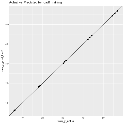
ggplot(data=plot_df_test_load1) + aes(x=test_y_actual, y=test_y_pred_load1) + geom_point() + geom_abline() + ggtitle("Actual vs Predicted for load1 test")
Of course we already knew what these were going to look like.
Fitting more models
Now let’s fit two more models, a random forest and a k-nearest neighbor (kNN), to really see how caret can facilitate rapid modeling. Both of these techniques have tuning parameters that we’ll let caret optimize. In addition, kNN requires data preprocessing since it relies on computing a distance between data points. Again, this isn’t meant to be an in-depth caret tutorial - we just want to show a few simple examples and then show how we can both automate and make the modeling process metadata driven.
For both of these techniques, let’s use a more general formula for the model. We will assume that the analyst is sufficiently knowledgeable of process physics that they incude the load and traffic intensity variables in addition to the arrival rate, average length of stay and capacity variables for the PP unit only.
Random forest
I’m just repeating (copy, paste, edit) what we did for the load1 model. Note that we are reusing the partitioned data as well as the trainControl object.
# Train a random forest
set.seed(resample_seed)
train_rf1 <- train(occmean_pp ~ lam_pp + alos_pp + cap_pp + load_pp + rho_pp,
                   data = obsim_train_df,
                   method = "rf",
                   trControl = fitControl)

# Make predictions
pred_rf1 <- predict(train_rf1, newdata = obsim_test_df)

# Summarize results
train_y_actual <- train_rf1$trainingData$.outcome
train_y_pred_rf1 <- fitted.values(train_rf1)

test_y_actual <- obsim_test_df[, "occmean_pp"]
test_y_pred_rf1 <- pred_rf1

rmse_train_rf1 <- rmse(train_y_actual, train_y_pred_rf1)
rmse_test_rf1 <- rmse(test_y_actual, test_y_pred_rf1)

plot_df_train_rf1 <- data.frame(train_y_actual, train_y_pred_rf1)
plot_df_test_rf1 <- data.frame(test_y_actual, test_y_pred_rf1)

cat(sprintf("rmse_train_rf1 = %0.5f\nrmse_test_rf1  = %0.5f \n",
            rmse_train_rf1, rmse_test_rf1))
## rmse_train_rf1 = 0.06760
## rmse_test_rf1 = 0.03202ggplot(data=plot_df_train_rf1) + aes(x=train_y_actual, y=train_y_pred_rf1) + geom_point() + geom_abline() + ggtitle("Actual vs Predicted for rf1 training")
ggplot(data=plot_df_test_rf1) + aes(x=test_y_actual, y=test_y_pred_rf1) + geom_point() + geom_abline() + ggtitle("Actual vs Predicted for rf1 test")
Hmm, that’s odd to get performance on test data that is better than on the training data. More on that later.
Let’s see what the best values of the tuning parameters optimized by caret. For the randomForest package, caret tries to find a good value for the mtry parameter (number of input variables “randomly sampled as candidates at each split”)
train_rf1$bestTune## mtry
## 3 5k nearest neighbors
I’m just repeating (copy, paste, edit) what we did for the rf1 model. However, we need specify one additional argument to the train function to tell caret to center and scale the data before fitting a kNN model. For kNN, caret will try to find a good value for \(k\).
# Train a kNN model
set.seed(resample_seed)
train_knn1 <- train(occmean_pp ~ lam_pp + alos_pp + cap_pp + load_pp + rho_pp,
                   data = obsim_train_df,
                   method = "knn",
                   trControl = fitControl,
                   preProcess=c("center", "scale"))

# Make predictions
pred_knn1 <- predict(train_knn1, newdata = obsim_test_df)

# Summarize results
train_y_actual <- train_knn1$trainingData$.outcome
train_y_pred_knn1 <- fitted.values(train_knn1)

test_y_actual <- obsim_test_df[, "occmean_pp"]
test_y_pred_knn1 <- pred_knn1

rmse_train_knn1 <- rmse(train_y_actual, train_y_pred_knn1)
rmse_test_knn1 <- rmse(test_y_actual, test_y_pred_knn1)

plot_df_train_knn1 <- data.frame(train_y_actual, train_y_pred_knn1)
plot_df_test_knn1 <- data.frame(test_y_actual, test_y_pred_knn1)

cat(sprintf("rmse_train_knn1 = %0.5f\nrmse_test_knn1  = %0.5f \n",
            rmse_train_knn1, rmse_test_knn1))
## rmse_train_knn1 = 1.21841
## rmse_test_knn1 = 0.04479ggplot(data=plot_df_train_knn1) + aes(x=train_y_actual, y=train_y_pred_knn1) + geom_point() + geom_abline() + ggtitle("Actual vs Predicted for knn1 training")
ggplot(data=plot_df_test_knn1) + aes(x=test_y_actual, y=test_y_pred_knn1) + geom_point() + geom_abline() + ggtitle("Actual vs Predicted for knn1 test")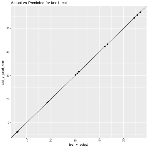
Again, strange to get better performance on test data then on training data. Makes me start to wonder about other things like:
- impact of different values for the number of folds and repeats in the k-crossfold process,
- training set size vs validation set size and on intervalidation set variability,
- impact of more modeling techniques such as neural networks and splines,
- impact of a “naive analyst” who might not think to include engineered features like load and traffic intensity,
- repeating the process for the other response variables,
- repeating all of this for the LDR unit,
- … and bunch more questions that are bound to be raised.
Just this little bit of copy, paste, editing was frought with errors and tediously repititious. Clearly we need to encapsulate this process in one or more functions. Ideally I also wanted to be able to create analysis scenarios defined by a bunch of attributes that I could store in a metadata file. To make this concrete, here’s a little csv file illustrating what I wanted to do.
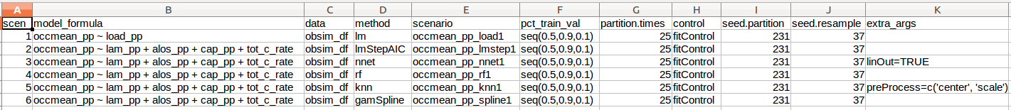 Here’s the actual csv file:
scenarios_test_df <- read.csv(file="data/scenarios_test.csv")
knitr::kable(scenarios_test_df)| scen | model_formula | data | method | scenario | pct_train_val | partition.times | control | seed.partition | seed.resample | extra_args |
|---|---|---|---|---|---|---|---|---|---|---|
| 1 | occmean_pp ~ load_pp | obsim_df | lm | occmean_pp_load1 | seq(0.5,0.9,0.1) | 10 | fitControl | 231 | 37 | |
| 2 | occmean_pp ~ lam_pp + alos_pp + cap_pp + tot_c_rate | obsim_df | lmStepAIC | occmean_pp_lmstep1 | seq(0.5,0.9,0.1) | 10 | fitControl | 231 | 37 | |
| 3 | occmean_pp ~ lam_pp + alos_pp + cap_pp + tot_c_rate | obsim_df | nnet | occmean_pp_nnet1 | seq(0.5,0.9,0.1) | 10 | fitControl | 231 | 37 | linout=TRUE |
| 4 | occmean_pp ~ lam_pp + alos_pp + cap_pp + tot_c_rate | obsim_df | rf | occmean_pp_rf1 | seq(0.5,0.9,0.1) | 10 | fitControl | 231 | 37 | |
| 5 | occmean_pp ~ lam_pp + alos_pp + cap_pp + tot_c_rate | obsim_df | knn | occmean_pp_knn1 | seq(0.5,0.9,0.1) | 10 | fitControl | 231 | 37 | preProcess=c(‘center’, ‘scale’) |
| 6 | occmean_pp ~ lam_pp + alos_pp + cap_pp + tot_c_rate | obsim_df | gamSpline | occmean_pp_spline1 | seq(0.5,0.9,0.1) | 10 | fitControl | 231 | 37 |
Next steps
I want to iterate through the rows of this dataframe and use the values to drive a set of model partition, train, predict and summarize cycles. What could possibly be so hard about that? Part 2 coming soon.
Reuse
Citation
@online{isken2016,
  author = {Isken, Mark},
  title = {Comparing Predictive Models for Obstetrical Unit Occupancy
    Using Caret - {Part} 1},
  date = {2016-06-24},
  url = {https://bitsofanalytics.org/posts/obsim-caret-1/obsim_caret_part1.html},
  langid = {en}
}