A vector-raster river map, three ways - Part 3: R

Using ggplot2, sf, terra, and friends to make maps

geonewb

mapping

geocomputation

Author

Mark Isken

Published

February 20, 2024

Background

In part 1 of this series we created a river map with QGIS and in part 2 with Python. We’ll finish it off with R. For the R based map, I decided to create a separate post written with Quarto to avoid messing around with the r2py package within Jupyter notebooks.

This finished products still need a lot of work. We are really just focusing on getting started with creating maps that combine vector and raster data and that require some combination of clipping, resampling and reprojecting. Along the way we’ll learn about some of the key R packages for working with geospatial data such as sf, terra and tidyterra. Most of the mapping will be done with ggplot2.

A few key online books I used include:

Geocomputation in R - extremely informative online book
The maps chapter in the ggplot2 book - ggplot2 has a wealth of built in mapping capabilities
R as GIS for Economists - another good online book

Data sources

The data, all freely available, is described in more detail in the first two posts in this series. It’s a combination of vector and raster data.

# Set environmental variable in $HOME/.Renviron
WSFR_DATA_ROOT <- Sys.getenv(c("WSFR_DATA_ROOT"))

Sites and basins (vector)

The streamflow guage sites and associated watershed basins are defined in the geospatial.gpkg GeoPackage file available from the WSFR data downloads page. GeoPackage files can contain multiple layers of both vector and raster data.

Under the hood, a GeoPackage is a SQLite database that conforms to the GeoPackage standard developed by the Open Geospatial Consortium. Both basins and sites are tables in the GeoPackage (SQLite database) and can be accessed directly with a SQLite database browser or any tool for working with SQLite databases.

In order to open a GeoPackage in R, we can use the simple features package.

library(sf)

Linking to GEOS 3.10.2, GDAL 3.4.1, PROJ 8.2.1; sf_use_s2() is TRUE

GEOS, GDAL and PROJ are all geospatial related system libraries used by the various R (and Python) geospatial packages. The fact that sf_use_s2() returns true, means that the s2 spherical geometry package is used. The R s2 package is a set of bindings to Google’s S2 package.

To read a GeoPackage file into R, we use the sf::st_read() function. Many functions in sf with begin with st_. We need to pass in the layer name since the file contains multiple layers.

basins_sf <- st_read(file.path(WSFR_DATA_ROOT, "geospatial.gpkg"), layer = "basins")

Reading layer `basins' from data source 
  `/home/mark/Documents/projects/driven_data/wsfrodeo/data/geospatial.gpkg' 
  using driver `GPKG'
Simple feature collection with 26 features and 3 fields
Geometry type: MULTIPOLYGON
Dimension:     XY
Bounding box:  xmin: -122.3289 ymin: 35.69785 xmax: -104.7031 ymax: 51.33442
Geodetic CRS:  WGS 84

sites_sf <- st_read(file.path(WSFR_DATA_ROOT, "geospatial.gpkg"), layer = "sites")

Reading layer `sites' from data source 
  `/home/mark/Documents/projects/driven_data/wsfrodeo/data/geospatial.gpkg' 
  using driver `GPKG'
Simple feature collection with 26 features and 2 fields
Geometry type: POINT
Dimension:     XY
Bounding box:  xmin: -122.2974 ymin: 35.70835 xmax: -104.718 ymax: 48.73217
Geodetic CRS:  WGS 84

In Python we used GeoPandas to create GeoDataFrame objects. An sf object is a geodataframe in an R sense - it’s a geospatially aware DataFrame object.

basins_sf

Simple feature collection with 26 features and 3 fields
Geometry type: MULTIPOLYGON
Dimension:     XY
Bounding box:  xmin: -122.3289 ymin: 35.69785 xmax: -104.7031 ymax: 51.33442
Geodetic CRS:  WGS 84
First 10 features:
                          site_id                                name      area
1   hungry_horse_reservoir_inflow       Hungry Horse Reservoir Inflow  1681.780
2                snake_r_nr_heise              Snake River near Heise  5719.410
3         pueblo_reservoir_inflow             Pueblo Reservoir Inflow  4615.460
4          sweetwater_r_nr_alcova        Sweetwater River near Alcova  2377.280
5            missouri_r_at_toston            Missouri River at Toston 14676.200
6             animas_r_at_durango             Animas River at Durango   700.901
7              yampa_r_nr_maybell            Yampa River near Maybell  3381.680
8          libby_reservoir_inflow              Libby Reservoir Inflow  9030.450
9                boise_r_nr_boise              Boise River near Boise  2687.340
10 green_r_bl_howard_a_hanson_dam Green River below Howard Hanson Dam   221.234
                             geom
1  MULTIPOLYGON (((-113.097 47...
2  MULTIPOLYGON (((-110.792 44...
3  MULTIPOLYGON (((-105.6734 3...
4  MULTIPOLYGON (((-107.3282 4...
5  MULTIPOLYGON (((-110.63 46....
6  MULTIPOLYGON (((-107.8758 3...
7  MULTIPOLYGON (((-107.028 40...
8  MULTIPOLYGON (((-114.8582 4...
9  MULTIPOLYGON (((-115.2353 4...
10 MULTIPOLYGON (((-121.3147 4...

Let’s plot these using ggplot2 just to get a sense of them. The geom_sf() function makes it easy to plot simple features.

library(ggplot2)

ggplot() +
    geom_sf(data = sites_sf, size = 2, shape = 23, fill = "#3399FF")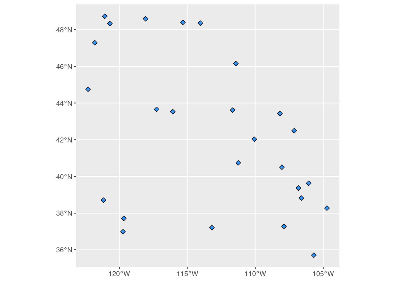

Notice we automatically get lat/lon values on the axes.

ggplot() +
    geom_sf(data = sites_sf, size = 2, shape = 23, fill = "#3399FF") +
    geom_sf(data = basins_sf, fill = "#a2d572")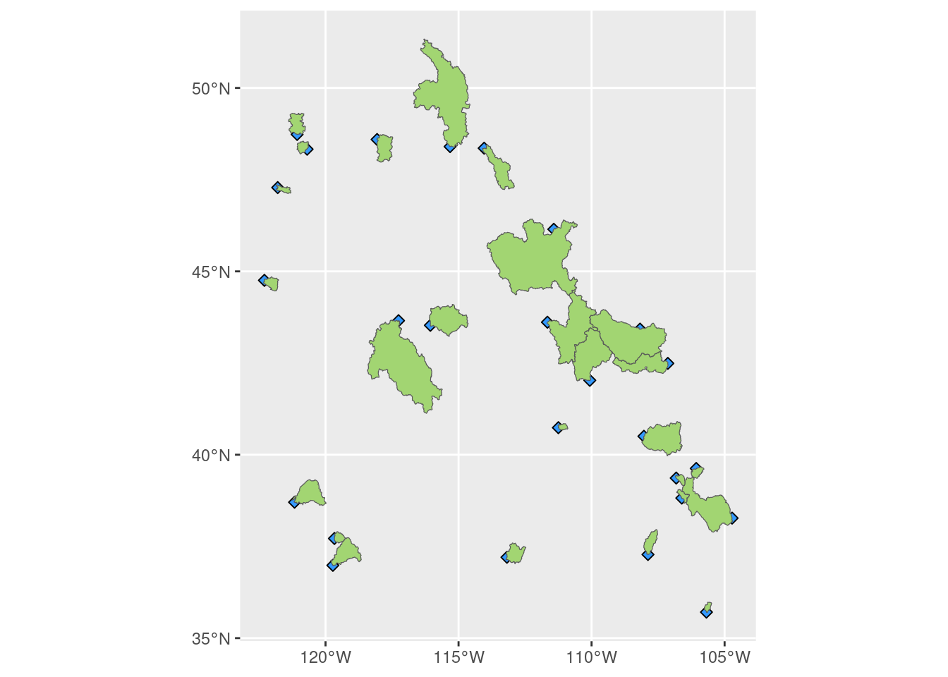

If we don’t want the grey background, we can use a different theme.

ggplot() +
    geom_sf(data = sites_sf, size = 2, shape = 23, fill = "#3399FF") +
    geom_sf(data = basins_sf, fill = "#a2d572") + 
    theme_classic()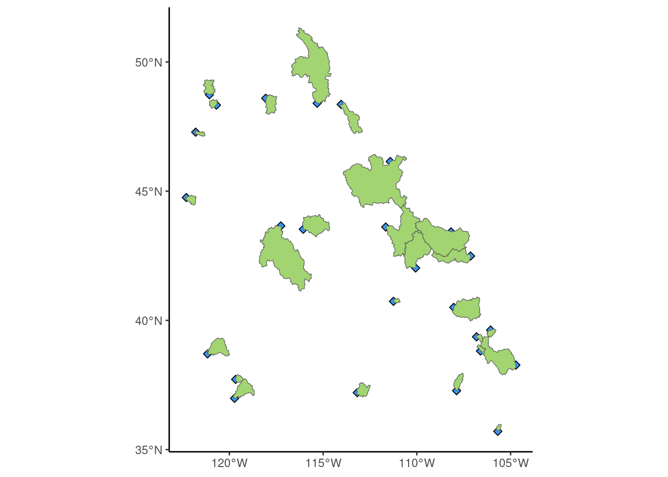

State and provincial boundaries (vector)

For this we can use the rnaturalearth package. It provides easy access to a whole lot of free vector and raster data focusing on our earth.

library(rnaturalearth)

NOTE After installing sf and rnaturalearth, both gave errors when I tried to load them with some message about a corrupted database. Quiting R Studio and restarting it resolved the problem. I think it’s something related to communication with the system PROJ library.

In order to plot more detailed maps, we need to install the rnaturalearthhires package from GitHub. To do this I needed the devtools package but when installing it the usual way I got issues due to missing system libraries - see https://github.com/r-lib/devtools/issues/2472. Not a big deal, but noticed in Hadley Wickham’s answer to this issue he suggested using writeLines(pak::pkg_system_requirements("devtools", "ubuntu", "22.04")) to see the exact dependencies. Hmm, that seems useful but I had not heard of the pak package before. Looks like it’s a new take on package management in R. So, did an install.packages("pak") (yep, old package manager to install new package manager package) and then pak::pkg_install("devtools") which led to really nice error messages telling me exactly which Ubuntu system libraries I needed to install manually.

sudo apt install libfribidi-dev libgit2-dev libharfbuzz-dev

Then redid the pak::pkg_install("devtools") followed by pak::pkg_install("ropensci/rnaturalearthhires"). Nice.

Let’s combine maps of states and provinces in the US and Candada into a single simple feature. The st_union() function makes this easy.

states_provinces_sf = st_union(ne_states(country = "united states of america"),
                                ne_states(country = "canada"))

ggplot() +
  geom_sf(data = states_provinces_sf["geometry"])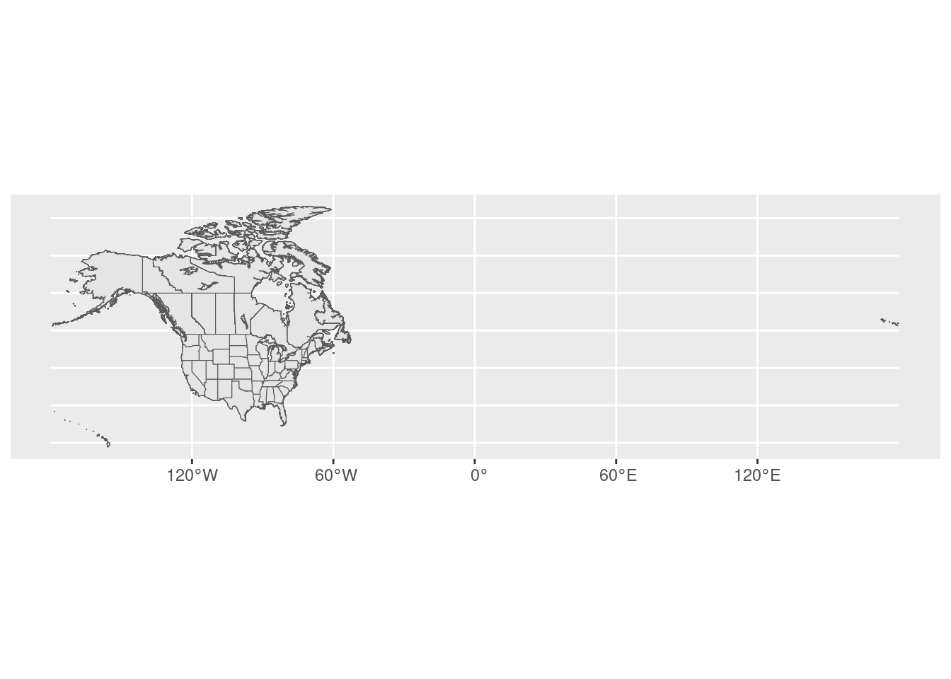

To set the map extent for the entire presentation layer, we can use the xlim= and ylim= arguments to coord_sf. Make sure that this is done after adding the map layers.

minx = -126
miny = 35
maxx = -103
maxy = 52

ggplot() +
  geom_sf(data = states_provinces_sf["geometry"]) +
  geom_sf(data = sites_sf, size = 2, shape = 23, fill = "#3399FF") +
  geom_sf(data = basins_sf, fill = "#a2d572") +
  coord_sf(xlim=c(minx, maxx), ylim=c(miny, maxy)) +
  theme_classic()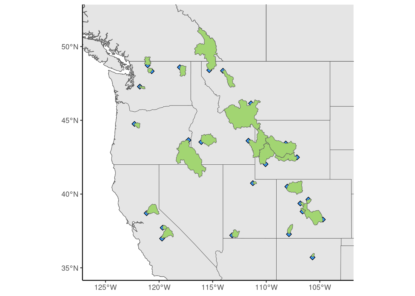

Now let’s change the CRS for the to Albers Equal Area using the ESRI:102008 code. We can use coord_sf to set the CRS. Under the hood, I imagine coord_sf is using the PROJ that is installed on your system and that was linked to when we loaded the sf library. I was hoping I could first set the map extent using EPSG:4326 limits and then change the CRS. But, this doesn’t work. Later we’ll convert all of the simple features to ESRI:102008 and do some other manipulations to plot just the area we are interested in.

This is not the right approach.

ggplot() +
  geom_sf(data = states_provinces_sf["geometry"]) +
  geom_sf(data = sites_sf, size = 2, shape = 23, fill = "#3399FF") +
  geom_sf(data = basins_sf, fill = "#a2d572") +
  coord_sf(xlim=c(minx, maxx), ylim=c(miny, maxy)) +
  coord_sf(crs = 'ESRI:102008') +
  theme_classic()

Coordinate system already present. Adding new coordinate system, which will
replace the existing one.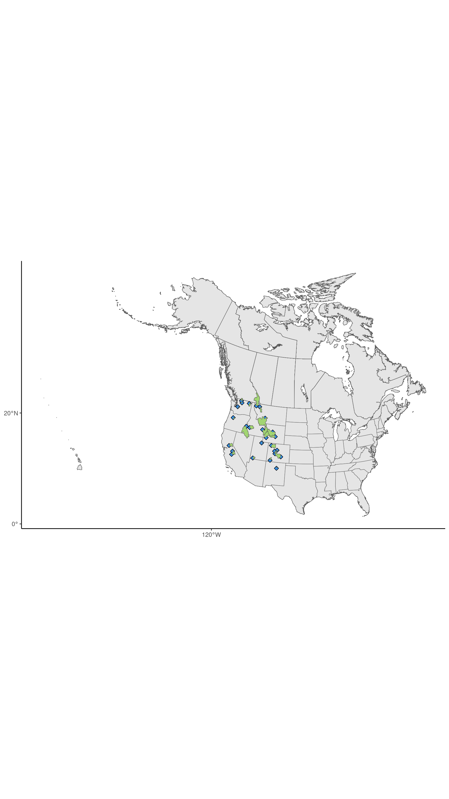

River layer (vector)

For this layer we can use HydroRIVERS data, a part of the HydroSHEDS project. Both geodatase and shapefile formats are downloadable from https://www.hydrosheds.org/products/hydrorivers. There are different files for different regions of the world. The North American and Central America data as a zipped geodatabase is available from here and is ~72Mb in size (compressed). Unzip it after downloading. It’s a lot of rivers.

A few tutorials I found on mapping rivers basins in R, include:

rivers_sf <- st_read(file.path(WSFR_DATA_ROOT, "hydrosheds/HydroRIVERS_v10_na.gdb", "HydroRIVERS_v10_na.gdb"))

Reading layer `HydroRIVERS_v10_na' from data source 
  `/home/mark/Documents/projects/driven_data/wsfrodeo/data/hydrosheds/HydroRIVERS_v10_na.gdb/HydroRIVERS_v10_na.gdb' 
  using driver `OpenFileGDB'
Simple feature collection with 986463 features and 15 fields
Geometry type: MULTILINESTRING
Dimension:     XY
Bounding box:  xmin: -137.9354 ymin: 5.510417 xmax: -52.66458 ymax: 62.67292
Geodetic CRS:  WGS 84

Now let’s filter by flow order and clip to a bounding box. The sf package includes the st_bbox() function for creating bounding boxes in a specific CRS. It also includes the st_crop() function for cropping simple features to a bounding box.

library(dplyr, warn.conflicts = FALSE)

rivers_sf <- rivers_sf %>% 
  filter(ORD_FLOW <= 5)

bbox <- st_bbox(c(xmin = minx, xmax = maxx, ymin = miny, ymax = maxy),
                crs = st_crs(basins_sf))

rivers_sf <- st_crop(rivers_sf, bbox)

Warning: attribute variables are assumed to be spatially constant throughout
all geometries

It seems that the placement of the coord_sf command is important. If I put it before the geom_sf layers, the extent of those layers seems to override the xlim and ylim values set in the coord_sf statement. It also seems important to express the limits so that they are consistent with the CRS used for the map.

ggplot() +
  geom_sf(data = states_provinces_sf) +
  geom_sf(data = sites_sf, size = 2, shape = 23, fill = "#3399FF") +
  geom_sf(data = basins_sf, fill = "#a2d572") +
  geom_sf(data = rivers_sf, color = "#487bb6") +
  coord_sf(xlim=c(minx, maxx), ylim=c(miny, maxy)) +
  theme_classic()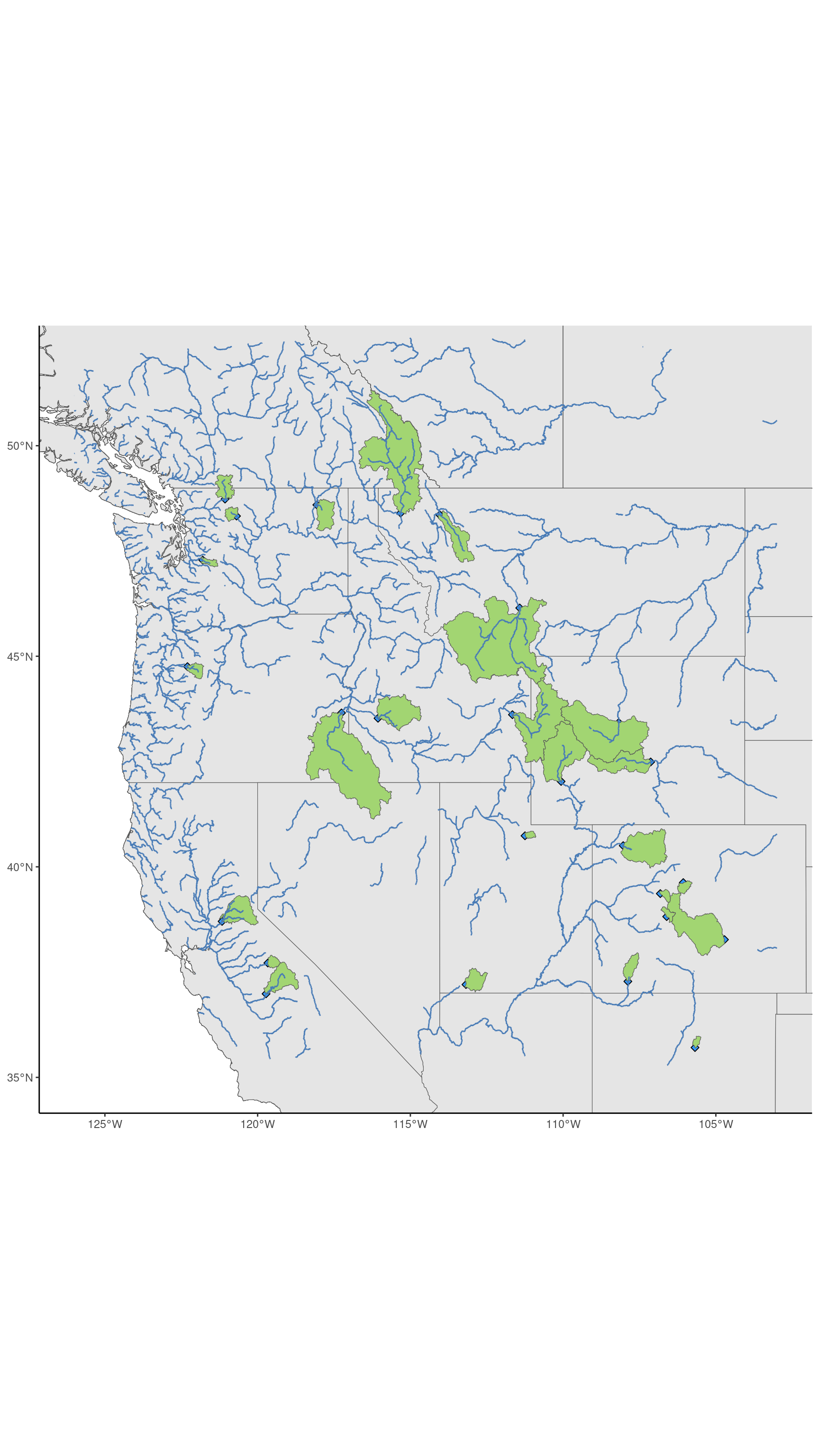

Digital Elevation Model or DEM (raster)

For working with raster data in R, the terra package is replacing the raster package. But, there’s also the stars package (written by the authors of sf). We will use terra in this post. For information on transitioning from raster to terra or stars, see this pdf.

library(terra)

terra 1.7.65

Documentation for terra can be found here.

We can read in the Hydrosheds DEM using the terra function rast().

dem_file = file.path(WSFR_DATA_ROOT, 'hydrosheds/na_con_3s/na_con_3s.tif')
dem_sr = terra::rast(dem_file)

The terra package has a bunch of functions for working with SpatRaster, SpatVector and SpatExtent objects.

terra::nrow(dem_sr) # Number of rows

[1] 72000

terra::ncol(dem_sr) # Number of columns

[1] 120000

terra::res(dem_sr) # resolution

[1] 0.0008333333 0.0008333333

The units of resolution are degrees. The DEM is 3 arc seconds on each side. This is ~90 meters at the equator.

writeLines(terra::crs(dem_sr))

GEOGCRS["WGS 84",
    DATUM["World Geodetic System 1984",
        ELLIPSOID["WGS 84",6378137,298.257223563,
            LENGTHUNIT["metre",1]]],
    PRIMEM["Greenwich",0,
        ANGLEUNIT["degree",0.0174532925199433]],
    CS[ellipsoidal,2],
        AXIS["geodetic latitude (Lat)",north,
            ORDER[1],
            ANGLEUNIT["degree",0.0174532925199433]],
        AXIS["geodetic longitude (Lon)",east,
            ORDER[2],
            ANGLEUNIT["degree",0.0174532925199433]],
    ID["EPSG",4326]]

What about the total number of cells and the number of layers?

terra::ncell(dem_sr)

[1] 8.64e+09

terra::nlyr(dem_sr)

[1] 1

The ext function creates a SpatExtent object from a vector specifying xmin, xmax, ymin, and ymax. Instead of using the extent used above, we are going to add on a buffer of 10 degrees in each direction (except west). Hopefully this will help avoid the problems with reprojecting and ending up with a raster that didn’t cover the entire area of interest.

buffer <- 5
map_extent <- terra::ext(c(bbox$xmin, bbox$xmax, bbox$ymin, bbox$ymax))
raster_extent <- terra::ext(c(bbox$xmin, bbox$xmax + buffer, bbox$ymin - buffer, bbox$ymax + buffer))

Now we can use the raster_extent to crop our DEM.

dem_sr <- terra::crop(dem_sr, raster_extent)


|---------|---------|---------|---------|
=========================================

dem_sr

class       : SpatRaster 
dimensions  : 32400, 33600, 1  (nrow, ncol, nlyr)
resolution  : 0.0008333333, 0.0008333333  (x, y)
extent      : -126, -98, 30, 57  (xmin, xmax, ymin, ymax)
coord. ref. : lon/lat WGS 84 (EPSG:4326) 
source      : spat_nthHTgVe8dNXZZB_10907.tif 
varname     : na_con_3s 
name        : Band_1 
min value   :  -1000 
max value   :   4363

terra::nrow(dem_sr)

[1] 32400

terra::ncol(dem_sr)

[1] 33600

terra::ncell(dem_sr)

[1] 1088640000

Adding the DEM raster to our plot

The ggplot2 package directly supports plotting vector data stored in sf objects through its geom_sf() and coord_sf() functions. The ggspatial library fills in some gaps to make plotting with ggplot2 easier and more powerful. We’ll also make use of tidyterra, a library that extends terra with tidyverse functions.

tidyterra

library(tidyterra, warn.conflicts = FALSE)

The two main stated goals of tidyterra are to:

add common tidyverse methods to SpatVector and SpatRaster objects (terra),
provide geoms to plot SpatVector and SpatRaster objects with ggplot2.

There is an article on tidyterra in the Journal of Open Source Software.

According to the docs for geom_spatraster(), it’s based on the layer_spatial() implementation in ggspatial. And, geom_spatvector() is a wrapper for ggplot2::geom_sf().

When you plot a SpatRaster with ggplot2 using geom_spatraster(), resampling is done automatically based on the number of cells in the raster.

This post by the author of tidyterra, has a nice discussion of issues surrounding choice of color gradients for elevation plots. For example, green connotes forest and so for the west we don’t want a linear scale with green for low values because too much will be green. A non-linear scale is more appropriate. The tidyterra package includes a number of such color gradients. The gradients are from [cpt-city] (http://soliton.vm.bytemark.co.uk/pub/cpt-city/), which is a huge collection of color gradient scales. Another good post on hillshade effect is this one by Dominic Roye.

From the pallets page, I chose the “etopo1_hypso” pallette, part of the hypso.colors2 collection of palletes.

grad_hypso <- hypso.colors2(10, "etopo1_hypso")

Now we are ready to add our DEM to the plot using geom_spatraster.

ggplot() +
  geom_spatraster(data = dem_sr) + scale_fill_gradientn(colours = grad_hypso, na.value = NA) +
  geom_sf(data = states_provinces_sf["geometry"], fill=NA) +
  geom_sf(data = sites_sf, size = 2, shape = 23, fill = "red") +
  geom_sf(data = basins_sf, fill = "green", alpha=0.20) +
  geom_sf(data = rivers_sf, color = "#487bb6") +
  coord_sf(crs = 'EPSG:4326', 
           xlim = c(map_extent$xmin, map_extent$xmax), ylim = c(map_extent$ymin, map_extent$ymax)) + 
  theme_classic()

<SpatRaster> resampled to 501095 cells for plotting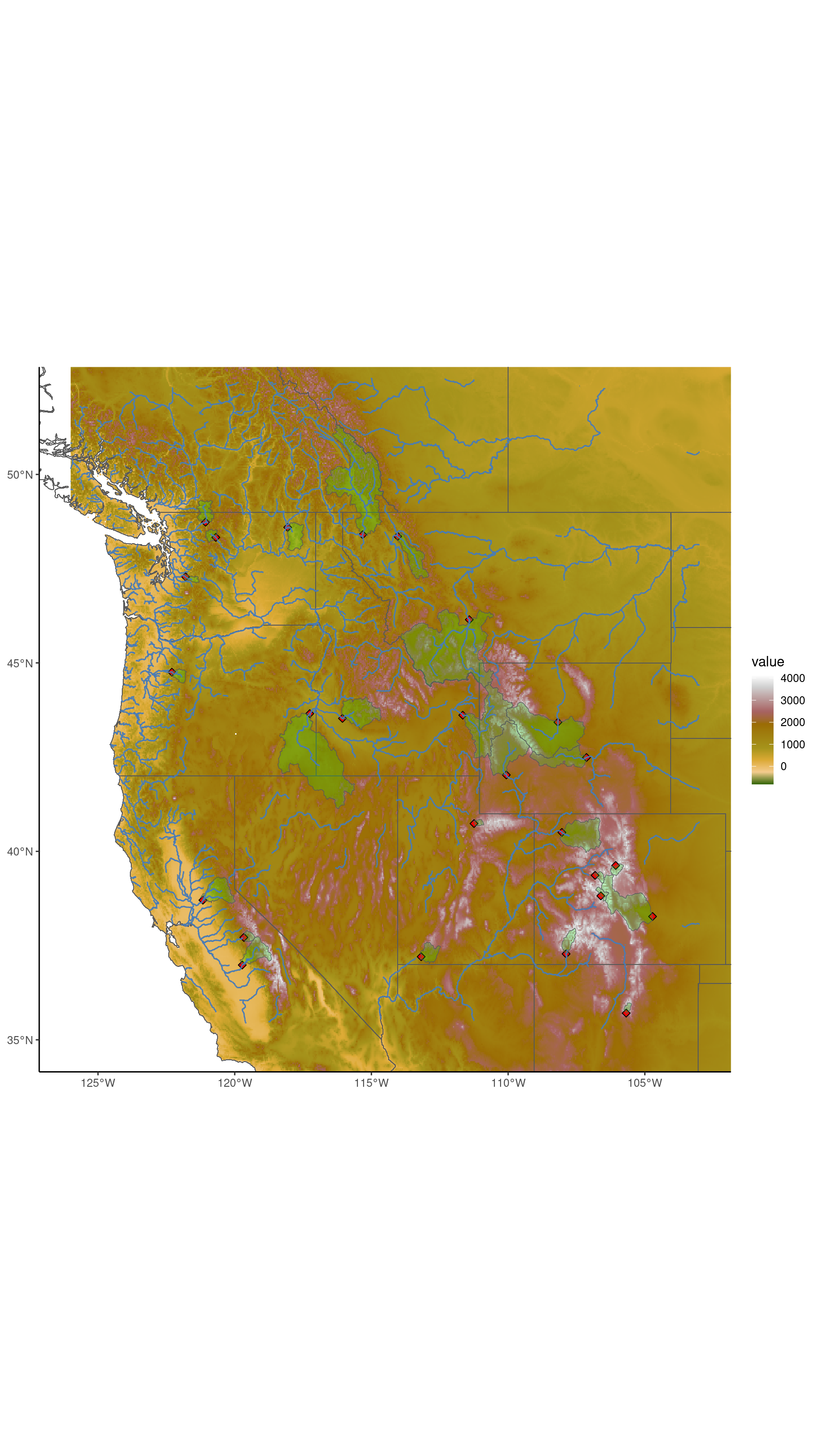

Reprojection

Our map is of a pretty big chunk of North America. Plotting directly as lat-lon values in the X-Y plane is probably not great in terms of distorting things like area and distance. Earlier we reprojected the state and province layer using Albers Equal Area (ESRI:102008). Let’s do that for all of the layers.

Here are

This section of GCwR is very good and has many links to relevant background sources:

Chapter 7 from the Geocomputation with R book,
How to specify a coordinate reference system in R
ECS530: (III) Coordinate reference systems - detailed history of PROJ, GDAL and their use in R and other systems.

Currently all of our data is in a geographic (non-projected) CRS - EPSG:4326. This CRS uses the WGS 94 datum as its ellipsoid model of the earth. The ESRI:102008 projection uses NAD83 as its datum. Good thing we’ve got tools to make it easy to convert between two such CRSs.

st_crs(rivers_sf)

Coordinate Reference System:
  User input: WGS 84 
  wkt:
GEOGCRS["WGS 84",
    ENSEMBLE["World Geodetic System 1984 ensemble",
        MEMBER["World Geodetic System 1984 (Transit)"],
        MEMBER["World Geodetic System 1984 (G730)"],
        MEMBER["World Geodetic System 1984 (G873)"],
        MEMBER["World Geodetic System 1984 (G1150)"],
        MEMBER["World Geodetic System 1984 (G1674)"],
        MEMBER["World Geodetic System 1984 (G1762)"],
        MEMBER["World Geodetic System 1984 (G2139)"],
        ELLIPSOID["WGS 84",6378137,298.257223563,
            LENGTHUNIT["metre",1]],
        ENSEMBLEACCURACY[2.0]],
    PRIMEM["Greenwich",0,
        ANGLEUNIT["degree",0.0174532925199433]],
    CS[ellipsoidal,2],
        AXIS["geodetic latitude (Lat)",north,
            ORDER[1],
            ANGLEUNIT["degree",0.0174532925199433]],
        AXIS["geodetic longitude (Lon)",east,
            ORDER[2],
            ANGLEUNIT["degree",0.0174532925199433]],
    USAGE[
        SCOPE["Horizontal component of 3D system."],
        AREA["World."],
        BBOX[-90,-180,90,180]],
    ID["EPSG",4326]]

The st_crs() function has a bunch of named items, including:

st_crs(new_vector)$IsGeographic to check is the CRS is geographic or not
st_crs(new_vector)$units_gdal to find out the CRS units
st_crs(new_vector)$srid to extract its ‘SRID’ identifier (when available)
st_crs(new_vector)$proj4string to extract the proj-string representation

st_crs(basins_sf)$IsGeographic

[1] TRUE

st_crs(basins_sf)$units_gdal

[1] "degree"

st_crs(basins_sf)$srid

[1] "EPSG:4326"

st_crs(basins_sf)$proj4string

[1] "+proj=longlat +datum=WGS84 +no_defs"

basins_102008_sf <- st_transform(basins_sf, "ESRI:102008")
sites_102008_sf <- st_transform(sites_sf, "ESRI:102008")
rivers_102008_sf <- st_transform(rivers_sf, "ESRI:102008")
states_provinces_102008_sf <- st_transform(states_provinces_sf, "ESRI:102008")

Notice how much more information is contained in the WKT (well known text) associated with ESRI:102008.

st_crs(basins_102008_sf)

Coordinate Reference System:
  User input: ESRI:102008 
  wkt:
PROJCRS["North_America_Albers_Equal_Area_Conic",
    BASEGEOGCRS["NAD83",
        DATUM["North American Datum 1983",
            ELLIPSOID["GRS 1980",6378137,298.257222101,
                LENGTHUNIT["metre",1]]],
        PRIMEM["Greenwich",0,
            ANGLEUNIT["Degree",0.0174532925199433]]],
    CONVERSION["North_America_Albers_Equal_Area_Conic",
        METHOD["Albers Equal Area",
            ID["EPSG",9822]],
        PARAMETER["Latitude of false origin",40,
            ANGLEUNIT["Degree",0.0174532925199433],
            ID["EPSG",8821]],
        PARAMETER["Longitude of false origin",-96,
            ANGLEUNIT["Degree",0.0174532925199433],
            ID["EPSG",8822]],
        PARAMETER["Latitude of 1st standard parallel",20,
            ANGLEUNIT["Degree",0.0174532925199433],
            ID["EPSG",8823]],
        PARAMETER["Latitude of 2nd standard parallel",60,
            ANGLEUNIT["Degree",0.0174532925199433],
            ID["EPSG",8824]],
        PARAMETER["Easting at false origin",0,
            LENGTHUNIT["metre",1],
            ID["EPSG",8826]],
        PARAMETER["Northing at false origin",0,
            LENGTHUNIT["metre",1],
            ID["EPSG",8827]]],
    CS[Cartesian,2],
        AXIS["(E)",east,
            ORDER[1],
            LENGTHUNIT["metre",1]],
        AXIS["(N)",north,
            ORDER[2],
            LENGTHUNIT["metre",1]],
    USAGE[
        SCOPE["Not known."],
        AREA["North America - onshore and offshore: Canada - Alberta; British Columbia; Manitoba; New Brunswick; Newfoundland and Labrador; Northwest Territories; Nova Scotia; Nunavut; Ontario; Prince Edward Island; Quebec; Saskatchewan; Yukon. United States (USA) - Alabama; Alaska (mainland); Arizona; Arkansas; California; Colorado; Connecticut; Delaware; Florida; Georgia; Idaho; Illinois; Indiana; Iowa; Kansas; Kentucky; Louisiana; Maine; Maryland; Massachusetts; Michigan; Minnesota; Mississippi; Missouri; Montana; Nebraska; Nevada; New Hampshire; New Jersey; New Mexico; New York; North Carolina; North Dakota; Ohio; Oklahoma; Oregon; Pennsylvania; Rhode Island; South Carolina; South Dakota; Tennessee; Texas; Utah; Vermont; Virginia; Washington; West Virginia; Wisconsin; Wyoming."],
        BBOX[23.81,-172.54,86.46,-47.74]],
    ID["ESRI",102008]]

st_crs(basins_102008_sf)$IsGeographic

[1] FALSE

st_crs(basins_102008_sf)$units_gdal

[1] "metre"

st_crs(basins_102008_sf)$srid

[1] "ESRI:102008"

st_crs(basins_102008_sf)$proj4string

[1] "+proj=aea +lat_0=40 +lon_0=-96 +lat_1=20 +lat_2=60 +x_0=0 +y_0=0 +datum=NAD83 +units=m +no_defs"

To reproject the raster DEM, we can use terra::project(). However, when i tried that it took forever and R died when I tried to kill the command. For reprojecting large rasters, using gdalwarp is often a good way to go. According to the documentation for the R package, gdalUtils, the sf package contains the GDAL executables along with R wrappers for them. The gdalUtilities package provides different wrappers whose arguments more closely match the GDAL executables.

# takes forever
#dem_102008_sr = terra::project(dem_sr, 'ESRI:102008')

library(gdalUtilities)


Attaching package: 'gdalUtilities'

The following object is masked from 'package:sf':

    gdal_rasterize

Since we had issues in the Python river map post related to the raster being clipped in unexpected ways, let’s take an alternative approach. Let’s try this:

use gdalUtilities to resample and reproject the clipped DEM raster to ESRI:102008 and write it to a file,
read the new file in using terra,
(maybe) clip the new raster by matching the extent of one of the existing vector layers.

The argument names used match those used by the gdalwarp command line tool.

r='bilinear' - the resampling algorithm (nearest neighbor is default),
tr = c(1000, 1000) - width and height of each pixel in units of the target SRS (spatial reference system),
te = ... - xmin, ymin, xmax, ymax of target extent,
te_srs = 'EPSG:4326', - the SRS corresponding to the te argument (avoid having to know the desired extent for the target SRS),
t_srs = 'ESRI:102008' - the target SRS

dem_file = file.path(WSFR_DATA_ROOT, 'hydrosheds/na_con_3s/na_con_3s.tif')
dem_102008_file = file.path(WSFR_DATA_ROOT, 'hydrosheds/na_con_3s/na_con_3s_102008_r.tif')

gdalUtilities::gdalwarp(dem_file, dem_102008_file, r = 'bilinear', tr = c(1000, 1000),
                        te = c(raster_extent$xmin, raster_extent$ymin, raster_extent$xmax, raster_extent$ymax),
                        te_srs = 'EPSG:4326',
                        t_srs = 'ESRI:102008',
                        overwrite = TRUE)

Let’s explore the new raster.

dem_102008_file = file.path(WSFR_DATA_ROOT, 'hydrosheds/na_con_3s/na_con_3s_102008_r.tif')
dem_102008_sr = terra::rast(dem_102008_file)

terra::nrow(dem_102008_sr)

[1] 2725

terra::ncol(dem_102008_sr)

[1] 2616

terra::ncell(dem_102008_sr)

[1] 7128600

Our DEM is much smaller now. We can use this new raster to extract a new map extent in meters for ESRI:102008.

map_extent_102008 <- ext(dem_102008_sr)
map_extent_102008

SpatExtent : -2735048.78302539, -119048.783025391, -731955.995255143, 1993044.00474486 (xmin, xmax, ymin, ymax)

Now use this SpatExtent to clip the state/province boundaries layer to the same size.

states_provinces_102008_sf <- st_crop(states_provinces_102008_sf, map_extent_102008)

Warning: attribute variables are assumed to be spatially constant throughout
all geometries

Okay, we’re ready to plot.

ggplot() +
  geom_spatraster(data = dem_102008_sr) + 
  scale_fill_gradientn(colours = grad_hypso, na.value = NA) +
  geom_sf(data = states_provinces_102008_sf["geometry"], fill=NA) +
  geom_sf(data = basins_102008_sf, aes(colour="Basins"),  alpha=0.20, fill="green", show.legend = "polygon") +
  geom_sf(data = sites_102008_sf, aes(colour="Sites"), size = 2, fill="red", shape = 23, show.legend = "point") + 
  scale_color_manual(values=c('green', 'red')) +
  geom_sf(data = rivers_102008_sf, color = "#487bb6") +
  coord_sf(crs = 'ESRI:102008', 
           xlim = c(map_extent_102008$xmin, map_extent_102008$xmax), 
           ylim = c(map_extent_102008$ymin, map_extent_102008$ymax)) + 
  theme_classic() +
  labs(title = "Water Supply Rodeo Forecast Sites")

<SpatRaster> resampled to 500346 cells for plotting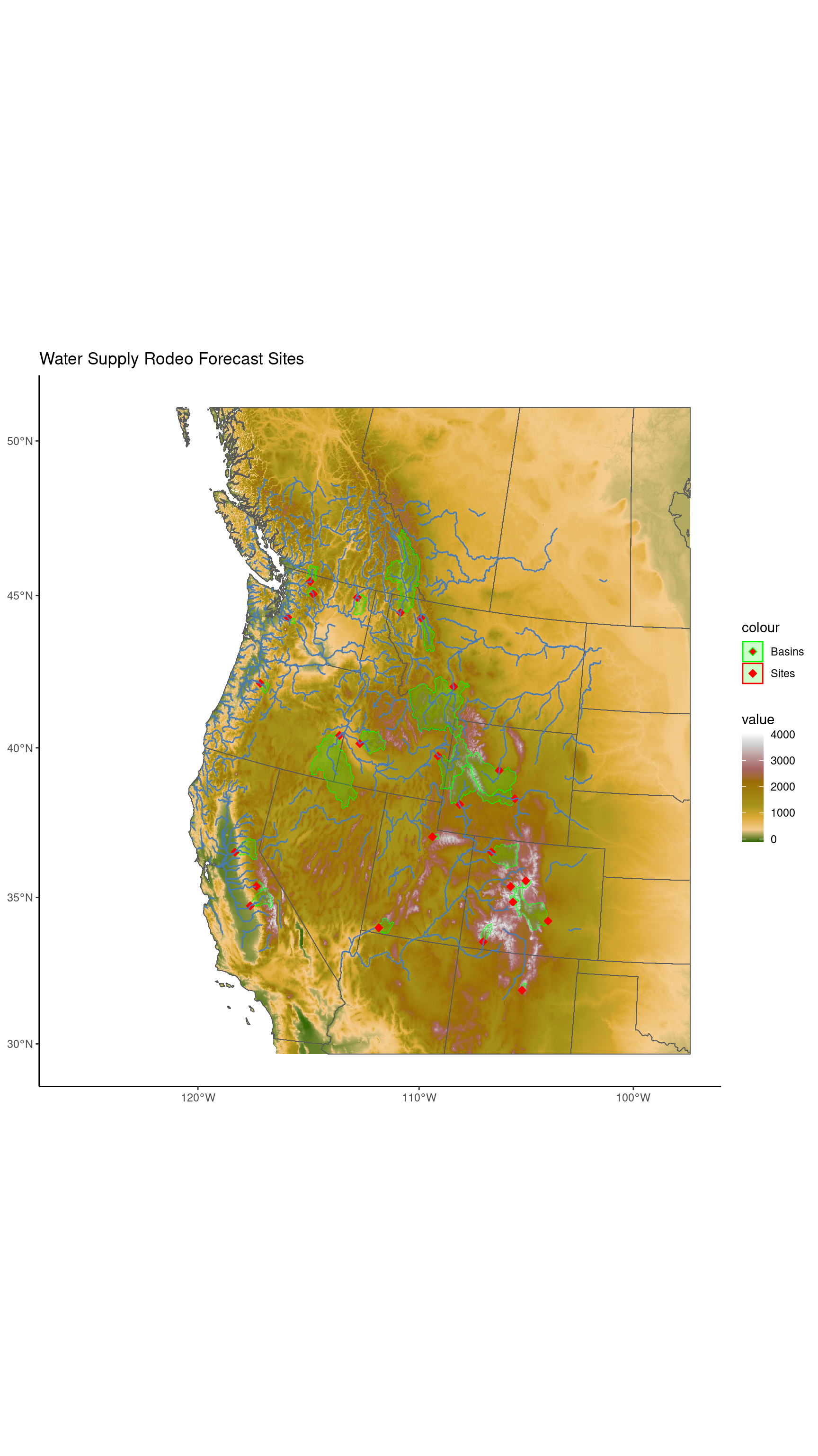

A few things to note:

the axis labels are in longitude and latitude as one would hope,
our raster has a colorbar legend entry,
the legend for the sites and basins is, not great. Not sure why both legend entries have red diamonds. Hmmm.

Seems there’s some trickiness with map legends in ggplot2. We’ll punt on this for now but leave some relevant links for future exploration.

Scale

Let’s end this post by adding a distance scale using the ggspatial package.

library(ggspatial)

ggplot() +
  geom_spatraster(data = dem_102008_sr) + 
  scale_fill_gradientn(colours = grad_hypso, na.value = NA) +
  geom_sf(data = states_provinces_102008_sf["geometry"], fill=NA) +
  geom_sf(data = basins_102008_sf, aes(colour="Basins"),  alpha=0.20, fill="green", show.legend = "polygon") +
  geom_sf(data = sites_102008_sf, aes(colour="Sites"), size = 2, fill="red", shape = 23, show.legend = "point") + 
  scale_color_manual(values=c('green', 'red')) +
  geom_sf(data = rivers_102008_sf, color = "#487bb6") +
  coord_sf(crs = 'ESRI:102008', 
           xlim = c(map_extent_102008$xmin, map_extent_102008$xmax), 
           ylim = c(map_extent_102008$ymin, map_extent_102008$ymax)) + 
  theme_classic() +
  labs(title = "Water Supply Rodeo Forecast Sites") +
  annotation_scale(location = "tl")

<SpatRaster> resampled to 500346 cells for plotting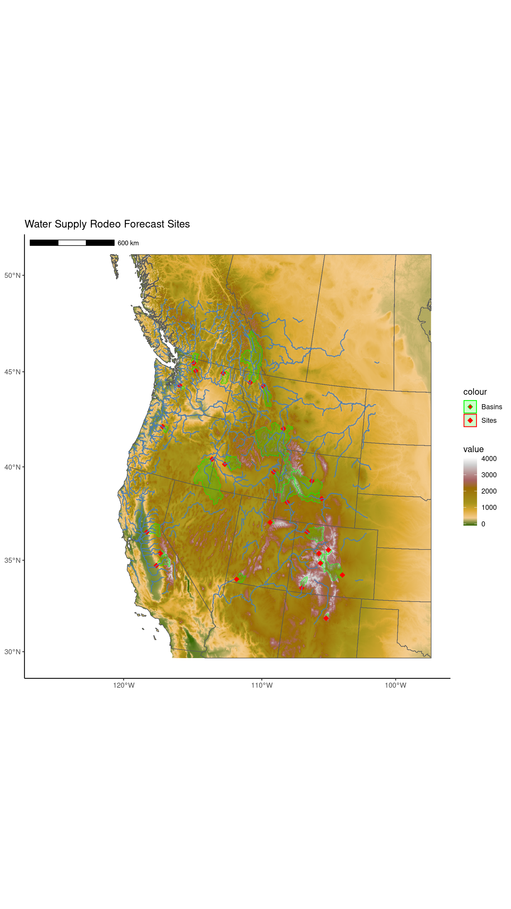

Seems like a good place to stop. Obviously, much to do in terms of getting all the details right to make really nice maps. But, we’ve at least figured out the basic workflow and relevant R packages for getting a first draft done.

Reuse

https://creativecommons.org/licenses/by/4.0/

Citation

BibTeX citation:

@online{isken2024,
  author = {Isken, Mark},
  title = {A Vector-Raster River Map, Three Ways - {Part} 3: {R}},
  date = {2024-02-20},
  langid = {en}
}

For attribution, please cite this work as:

Isken, Mark. 2024. “A Vector-Raster River Map, Three Ways - Part 3: R.” February 20, 2024.