library(dplyr)
library(ggplot2)
library(lubridate)Wednesday Birders 2018
Stats and plots using R
R
python
birding
In a previous post I described how I used a mix of Python and R to acquire, clean, and analyze eBird data from our birding group’s weekly walks. In this post, I’ll add plots for 2018 and do a little more analysis.
To summarize the basic approach (described in the first post), we:
- used the eBird API (2.0) with Python to download data from our bird lists into a pandas dataframe and then exported to csv file,
- used R to clean up the data to make sure we were just using our Wednesday Birders lists for the analysis,
- used the R packages dplyr and ggplot2 to summarize and make plots of species counts by year.
Data prep
All of the data prep and analysis is done in R. We’ll need a few libraries:
Before diving into analysis and plots, a little data prep was needed:
- downloaded data from 2018 and converted the JSON to csv (used appropriately modified Python script detailed in first post)
- read CSV file into an R dataframe
- convert datetime fields to POSIXct
- include only the lists from our Wednesday morning walks
- combined the 2018 data with the data from 2015-1017 and saved as an RDS file
obs_df <- readRDS(file = "./data/observations.rds")There are a bunch of fields in the observation records from eBird. Here’s just a sample focusing on the stuff we need. Each row in the data frame corresponds to an individual species count on a certain date in a certain location.
obs_df <- obs_df %>%
  select(checklistId, obsDt, locName, comName, sciName, howMany, subId)

head(obs_df)
checklistId obsDt locName comName
1 CL24105 2015-03-18 09:35:00 Charles Ilsley Park Canada Goose
2 CL24105 2015-03-18 09:35:00 Charles Ilsley Park Turkey Vulture
3 CL24105 2015-03-18 09:35:00 Charles Ilsley Park Red-tailed Hawk
4 CL24105 2015-03-18 09:35:00 Charles Ilsley Park Sandhill Crane
5 CL24105 2015-03-18 09:35:00 Charles Ilsley Park Red-bellied Woodpecker
6 CL24105 2015-03-18 09:35:00 Charles Ilsley Park Downy Woodpecker
sciName howMany subId
1 Branta canadensis 2 S22414352
2 Cathartes aura 1 S22414352
3 Buteo jamaicensis 2 S22414352
4 Antigone canadensis 2 S22414352
5 Melanerpes carolinus 1 S22414352
6 Picoides pubescens 1 S22414352Plots of Species Counts
How many birds of each species have we seen? How frequently are each species seen?
Let’s start with simple bar charts:
- one bar per species, one year per graph,
- bar length is number of birds seen,
- color of bar is related to percentage of lists on which that species seen,
- number at end of bar is percentage of lists on which that species seen.
Here are the plots from 2015-2017:
knitr::include_graphics("images/top30_2015.png")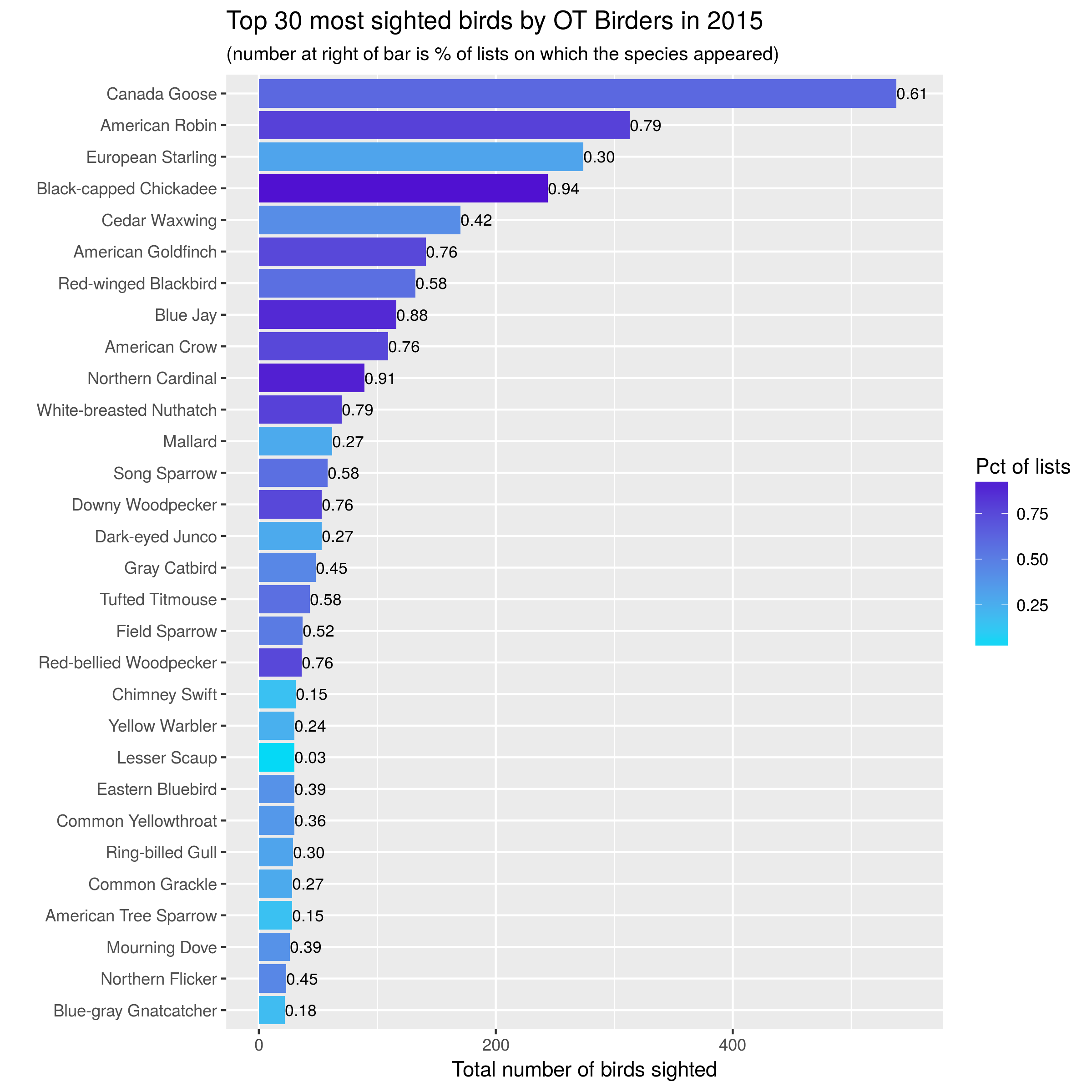
knitr::include_graphics("images/top30_2016.png")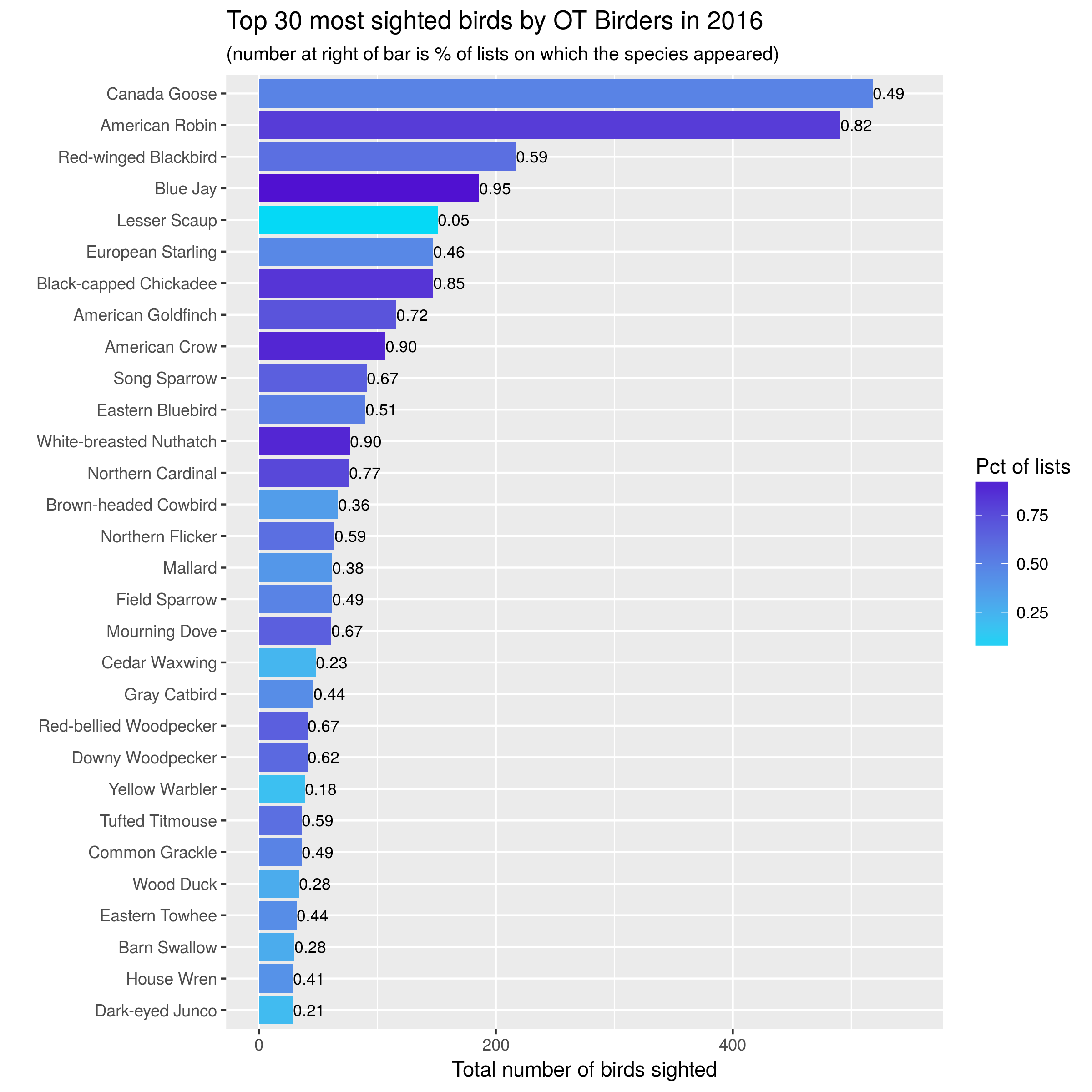
knitr::include_graphics("images/top30_2017.png")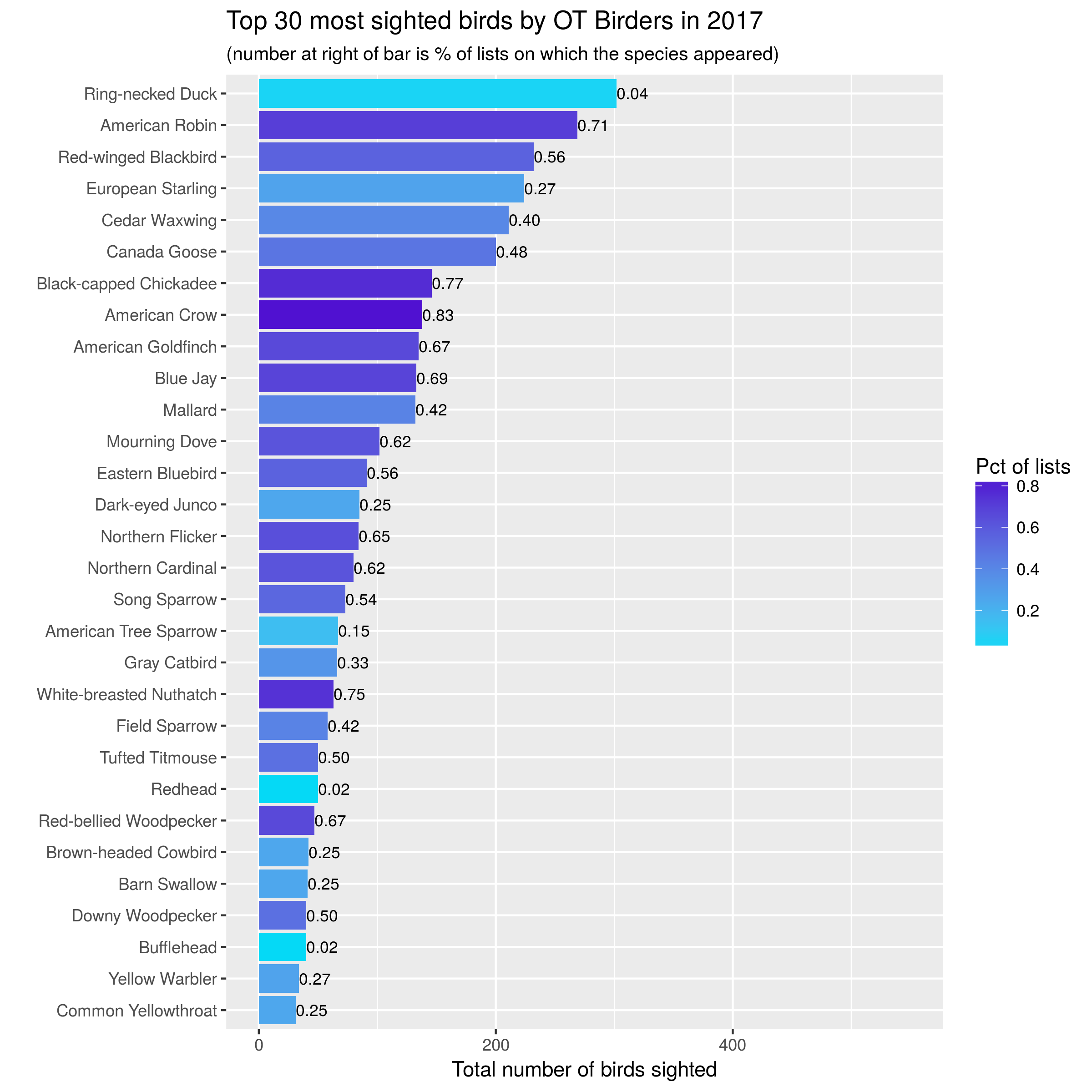
Creating the plot for 2018
`summarise()` has regrouped the output.
`summarise()` has regrouped the output.
ℹ Summaries were computed grouped by year, obsDt, locName, and subId.
ℹ Output is grouped by year, obsDt, and locName.
ℹ Use `summarise(.groups = "drop_last")` to silence this message.
ℹ Use `summarise(.by = c(year, obsDt, locName, subId))` for per-operation
  grouping (`?dplyr::dplyr_by`) instead.
The plots above are easy to create from a dataframe that looks like this:
                   comName birding_year num_lists tot_birds totlists   pctlists
1           American Robin         2018        32       466       41 0.78048780
2             Canada Goose         2018        23       239       41 0.56097561
3       American Goldfinch         2018        32       212       41 0.78048780
4     Red-winged Blackbird         2018        33       204       41 0.80487805
5            Mourning Dove         2018        35       176       41 0.85365854
6            Cedar Waxwing         2018        18       142       41 0.43902439
7                 Blue Jay         2018        41       139       41 1.00000000
8   Black-capped Chickadee         2018        41       125       41 1.00000000
9            American Crow         2018        36       106       41 0.87804878
10        Eastern Bluebird         2018        23        97       41 0.56097561
11       European Starling         2018        15        89       41 0.36585366
12       Northern Cardinal         2018        40        81       41 0.97560976
13            Song Sparrow         2018        26        81       41 0.63414634
14          Turkey Vulture         2018        17        52       41 0.41463415
15                 Mallard         2018        18        51       41 0.43902439
16        Ring-billed Gull         2018        12        51       41 0.29268293
17            Lesser Scaup         2018         1        50       41 0.02439024
18                 Redhead         2018         1        50       41 0.02439024
19         Dark-eyed Junco         2018        15        46       41 0.36585366
20         Tufted Titmouse         2018        26        45       41 0.63414634
21 White-breasted Nuthatch         2018        24        43       41 0.58536585
22          Common Grackle         2018        16        41       41 0.39024390
23  Red-bellied Woodpecker         2018        31        41       41 0.75609756
24        Downy Woodpecker         2018        27        38       41 0.65853659
25           Field Sparrow         2018        15        37       41 0.36585366
26             Rock Pigeon         2018         6        37       41 0.14634146
27            Barn Swallow         2018        12        36       41 0.29268293
28        Northern Flicker         2018        21        36       41 0.51219512
29            Tree Swallow         2018        11        35       41 0.26829268
30    Brown-headed Cowbird         2018        12        33       41 0.29268293
Here’s how you can make such a data frame.
# Create num species by list df
numsp_bylist <- obs_df %>%
  group_by(year=year(obsDt), obsDt, locName, subId) %>%
  summarize(
    n = n(),
    totbirds = sum(howMany)
  ) %>%
  arrange(year, subId)
`summarise()` has regrouped the output.
ℹ Summaries were computed grouped by year, obsDt, locName, and subId.
ℹ Output is grouped by year, obsDt, and locName.
ℹ Use `summarise(.groups = "drop_last")` to silence this message.
ℹ Use `summarise(.by = c(year, obsDt, locName, subId))` for per-operation
grouping (`?dplyr::dplyr_by`) instead.# Using numsp_bylist, create num lists by date
numlists_bydt <- numsp_bylist %>%
group_by(obsDt) %>%
summarise(
numlists = n()
) %>%
filter(numlists >= 1) %>%
arrange(obsDt)
# Usings numlists_bydt, create num lists by year
numlists_byyear <- numlists_bydt %>%
group_by(birding_year=year(obsDt)) %>%
summarise(
totlists = sum(numlists)
)
# Now ready to compute species by year
species_byyear <- obs_df %>%
group_by(comName, birding_year=year(obsDt)) %>%
summarize(
num_lists = n(),
tot_birds = sum(howMany)
) %>%
arrange(birding_year, desc(tot_birds))`summarise()` has regrouped the output.
ℹ Summaries were computed grouped by comName and birding_year.
ℹ Output is grouped by comName.
ℹ Use `summarise(.groups = "drop_last")` to silence this message.
ℹ Use `summarise(.by = c(comName, birding_year))` for per-operation grouping
(`?dplyr::dplyr_by`) instead.# Join to numlists_byyear so we can compute pct of lists each species
# appeared in.
species_byyear <- left_join(species_byyear, numlists_byyear, by = 'birding_year')
bird_year <- 2018
top_obs_byyear <- species_byyear %>%
filter(birding_year == bird_year) %>%
mutate(pctlists = num_lists / totlists) %>%
arrange(desc(tot_birds)) %>%
head(30)Make the plot.
ggplot(top_obs_byyear) +
    geom_bar(aes(x=reorder(comName, tot_birds),
                 y=tot_birds, fill=pctlists), stat = "identity") +
                 scale_fill_gradient(low='#05D9F6', high='#5011D1') +
                 labs(x="",
                      y="Total number of birds sighted",
                      fill="Pct of lists",
                      title = paste0("Top 30 most sighted birds by Wednesday Birders in ", bird_year),
                      subtitle = "(number at right of bar is % of lists on which the species appeared)") +
                 coord_flip() +
    geom_text(data=top_obs_byyear,
              aes(x=reorder(comName,tot_birds),
                  y=tot_birds,
                  label=format(pctlists, digits = 1),
                  hjust=0
              ), size=3) + ylim(0,500)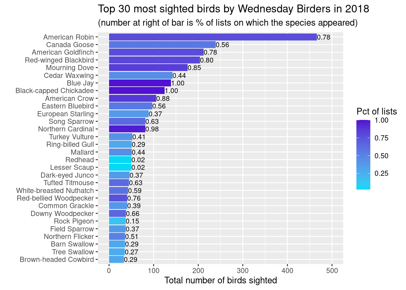
Patterns and changes over time
Now that we have four full years of eBird sightings data from the four parks we visit each month, let’s see how things look over time (and location).
Here’s an overall time series plot of number of species appearing on each list.
numsp_bylist %>%
  ggplot() + geom_point(aes(x = as.Date(obsDt), y = n)) +
  ggtitle("Number of species sighted for each list", subtitle = "2015-2018") +
  scale_x_date(date_breaks = "3 months",
               date_labels = "%m-%y") +
  xlab("List date (month-year)") +
  ylab("Number of species")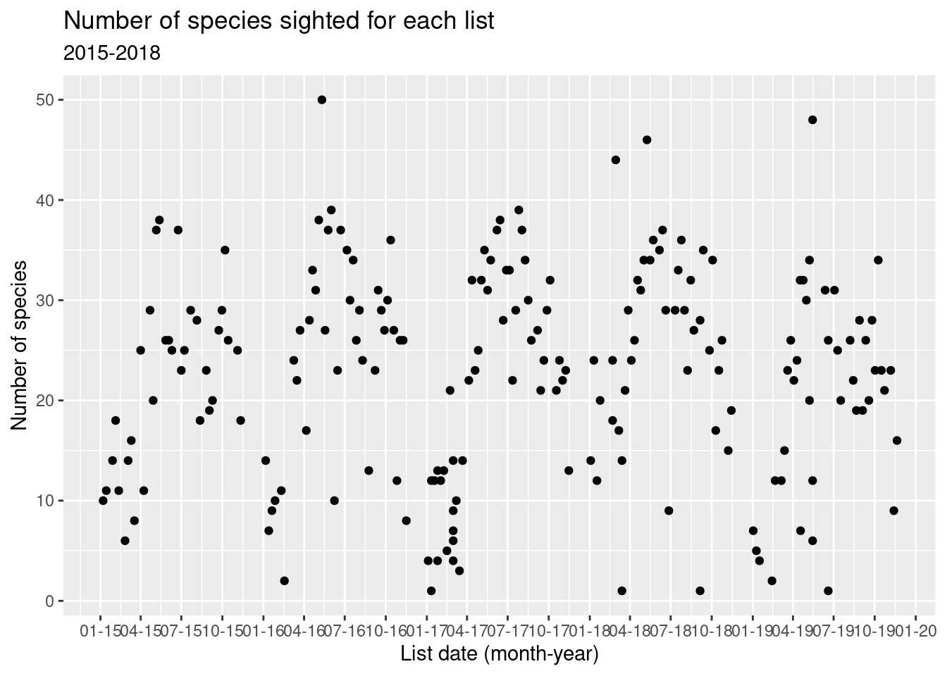
Same plot but faceted by park.
numsp_bylist %>%
  ggplot() + geom_point(aes(x = as.Date(obsDt), y = n)) +
  facet_grid(locName ~ .) +
  ggtitle("Number of species sighted for each list", subtitle = "2015-2018") +
  scale_x_date(date_breaks = "3 months",
               date_labels = "%m-%y") +
  xlab("List date (month-year)") +
  ylab("Number of species")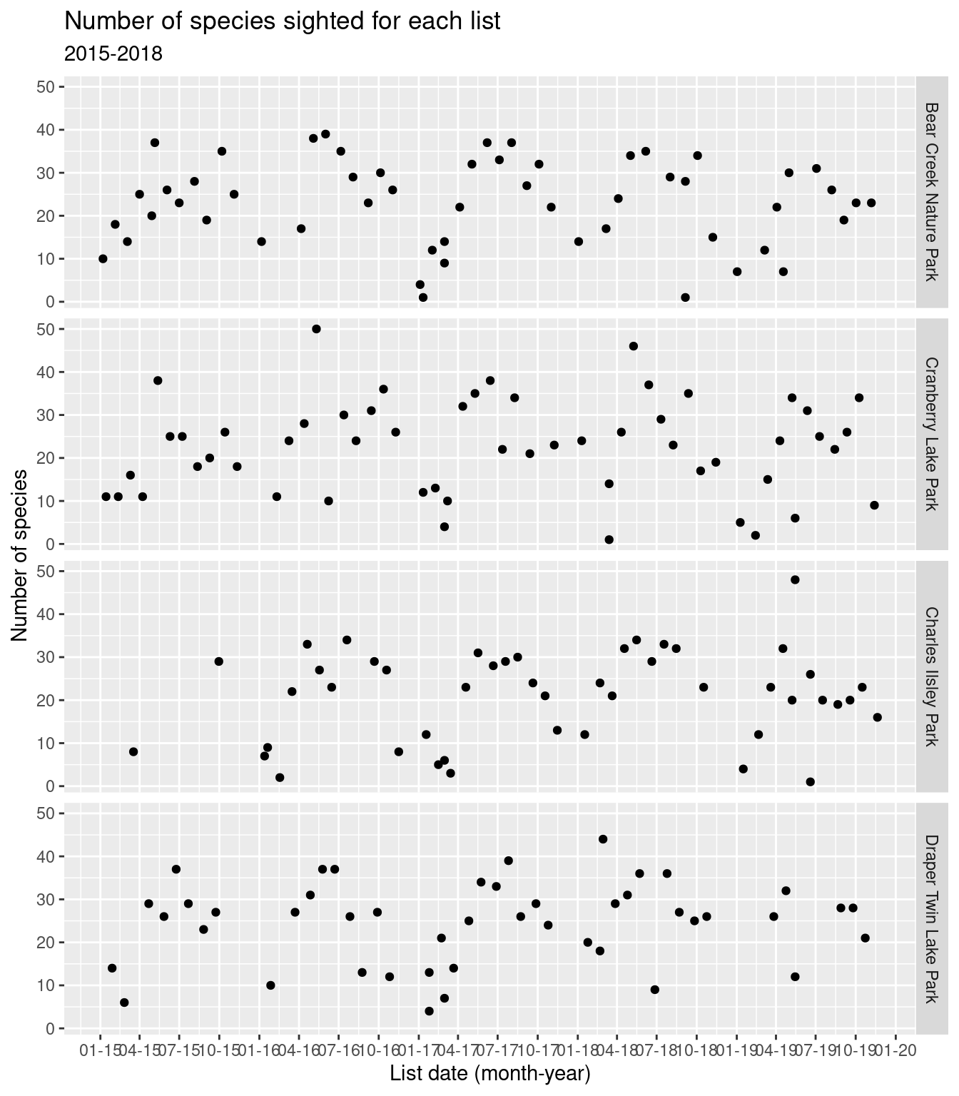
Let’s look at distribution of list size during the peak period of April-October.
numsp_bylist %>%
  filter(month(obsDt) %in% 4:10) %>%
  ggplot() + geom_histogram(aes(x = n, y = ..density..), bins = 20) +
  ggtitle("Distribution of list size", subtitle = "April-October") +
  xlab("List size (number of species)") +
  geom_density(aes(x = n))
Warning: The dot-dot notation (`..density..`) was deprecated in ggplot2 3.4.0.
ℹ Please use `after_stat(density)` instead.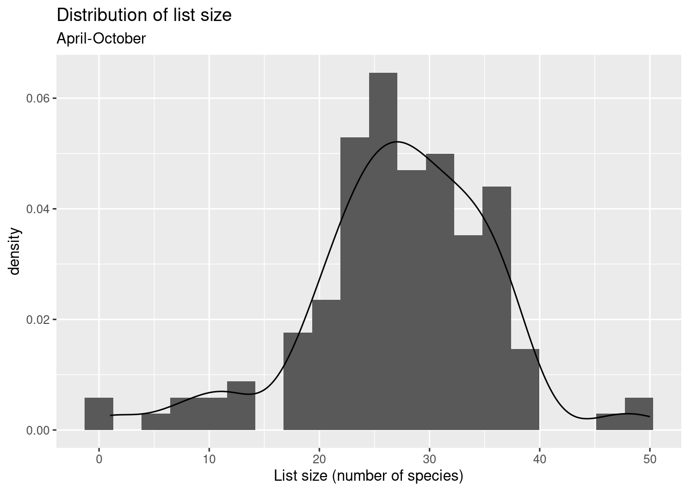
Use boxplots and group by park.
numsp_bylist %>%
  filter(month(obsDt) %in% 4:10) %>%
  ggplot() + geom_boxplot(aes(x = locName, y = n)) +
  ggtitle("Distribution of list size", subtitle = "April-October") +
  xlab("Location") + ylab("List size (number of species)")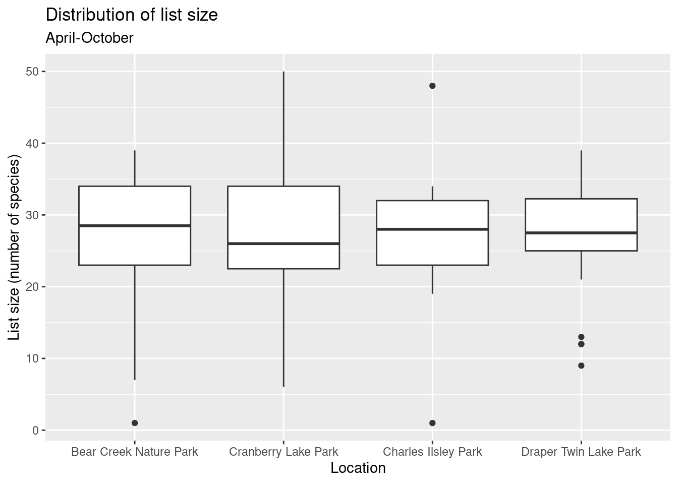
Let’s repeat the above but using total number of birds counted per list instead of number of species per list.
numsp_bylist %>%
  filter(month(obsDt) %in% 4:10) %>%
  ggplot() + geom_boxplot(aes(x = locName, y = totbirds)) +
  ggtitle("Distribution of number of total birds per list", subtitle = "April-October") +
  xlab("Location") + ylab("List size (number of birds counted)")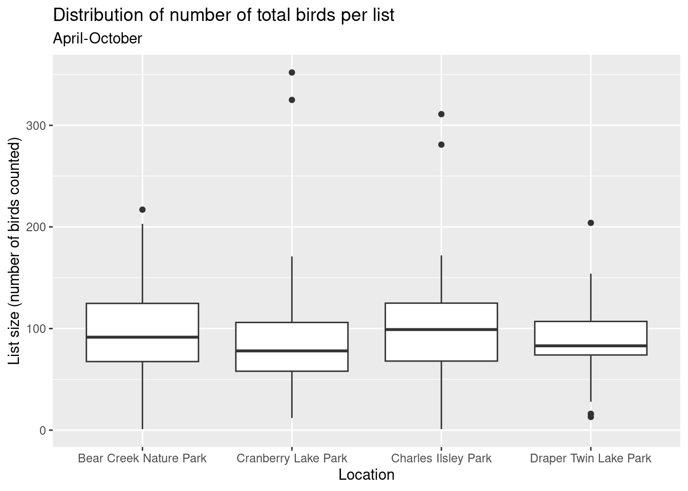
Let’s look at time series plots of number of birds counted for each of the species in the Top 30 for 2018. We’ll need the following data frame to power the plots.
top_species_byyear <- top_obs_byyear %>%
  select("comName") %>%
  inner_join(species_byyear, by = "comName") %>%
  mutate(pctlists = num_lists / totlists)

top_species_byyear
# A tibble: 143 × 6
# Groups: comName [30]
comName birding_year num_lists tot_birds totlists pctlists
<fct> <dbl> <int> <dbl> <int> <dbl>
1 American Robin 2015 26 313 33 0.788
2 American Robin 2016 32 491 39 0.821
3 American Robin 2017 34 269 48 0.708
4 American Robin 2018 32 466 41 0.780
5 American Robin 2019 33 390 41 0.805
6 Canada Goose 2015 20 538 33 0.606
7 Canada Goose 2016 19 518 39 0.487
8 Canada Goose 2017 23 200 48 0.479
9 Canada Goose 2018 23 239 41 0.561
10 Canada Goose 2019 22 395 41 0.537
# ℹ 133 more rowsBar height is total number of birds counted and bar color is related to percentage of lists on which this bird appeared.
ggplot(top_species_byyear) +
  geom_bar(aes(x = birding_year, y = tot_birds, fill=pctlists),
           stat = "identity") +
  scale_fill_gradient(low='#05D9F6', high='#5011D1') +
  ggtitle("Number of birds counted by year") +
  facet_wrap(~comName, ncol = 5, scales = "free_y") +
  labs(x="Year",
       y="Total number of birds sighted",
       fill="Pct of lists")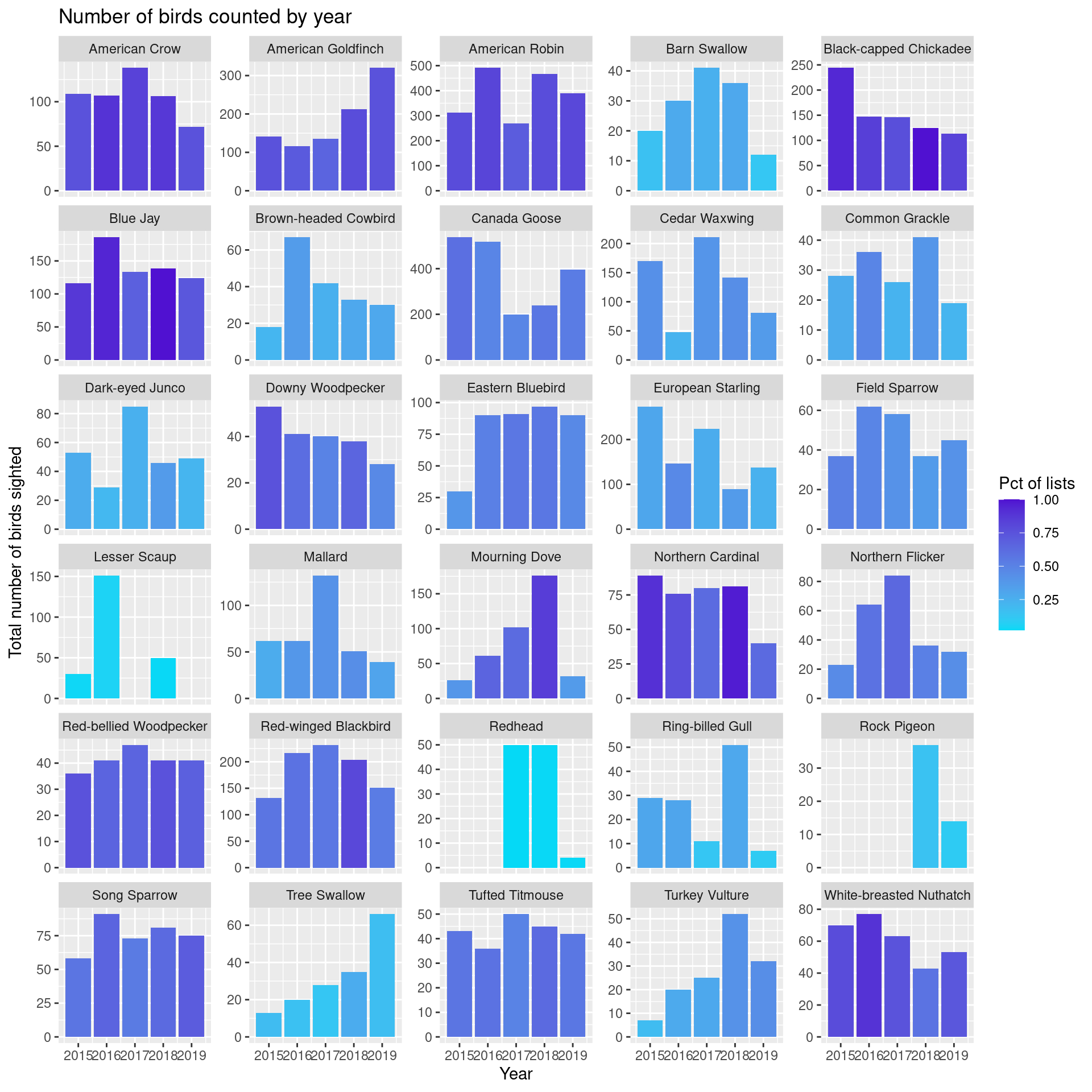
A few things pop out:
- overall number of Black-capped Chicadees counted has declined, though they are still sighted very frequently. Maybe we’ve become somewhat immune to their constant chatter and just aren’t recording as many. “Oh, just another chicadee.”
- Downy Woodpecker sightings have declined both in terms of number and frequency as have White-breasted Nuthatch sightings.
- Mourning Doves are up in both number and frequency.
- After 2015, sightings of Eastern Bluebirds have been remarkably constant.
Now swap roles of total birds and frequency of appearing on a list. Bar height is percentage of lists on which this bird appeared and bar color is related to total number of birds counted.
ggplot(top_species_byyear) +
  geom_bar(aes(x = birding_year, y = pctlists, fill = tot_birds),
           stat = "identity") +
  scale_fill_gradient(low='#05D9F6', high='#5011D1') +
  ggtitle("Number of birds counted by year") +
  facet_wrap(~comName, ncol = 5) +
  labs(x="Year",
       y="Pct of lists",
       fill="Total birds counted")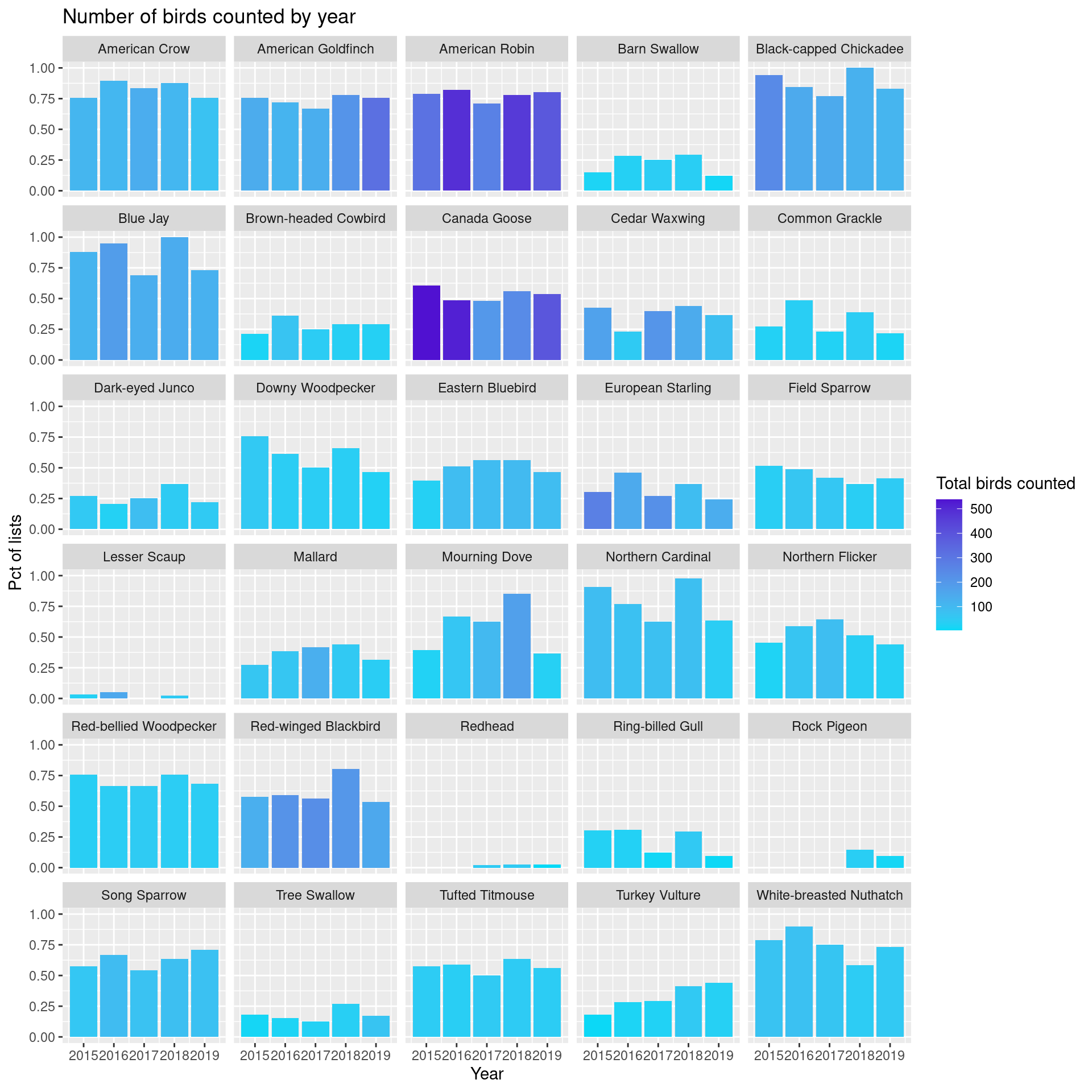
Next steps
Now our group can try to make sense of these and I’m sure we’ll have ideas for more analysis. In my next post I’m going to explore those springtime favorites, the warblers.
Reuse
Citation
BibTeX citation:
@online{isken2019,
  author = {Isken, Mark},
  title = {Wednesday {Birders} 2018},
  date = {2019-02-04},
  url = {https://bitsofanalytics.org/posts/otbirders-2-stats-2018/otbirders_2_stats_2018.html},
  langid = {en}
}
For attribution, please cite this work as:
Isken, Mark. 2019. “Wednesday Birders 2018.” February 4. https://bitsofanalytics.org/posts/otbirders-2-stats-2018/otbirders_2_stats_2018.html.