Using the ebird API, Python, and R to analyze data for our birding group
R
python
birding
Author
Mark Isken
Published
April 16, 2018
Since 2015, a small but growing group of birders has met each Wednesday morning to bird one of the parks in Oakland Township. We have a mix of birding experience, a shared love of nature and dedication to stewardship of natural areas. The founder of the group is a scientist/naturalist (PhD in biology/botany) and the Natural Areas Manager for Oakland Township. So, not only do we get to bird, we get to learn a ton about the flora of the area. Our group is also fortunate to have a gifted writer and photographer who blogs about our parks at the Natural Areas Notebook.
Since the group’s inception, our bird lists have been entered into eBird, making it easy to answer those “Hey, have we ever seen a [insert random bird species] in this park?” queries. Now that we’ve got a few years of weekly data, it’s time for some birding analysis. In this first post, I’ll describe how I:
used the eBird API (2.0) with Python from a Jupyter notebook to download data from our bird lists into a pandas dataframe and then exported to csv file,
used R to clean up the data to make sure we were just using our Wednesday Birders lists for the analysis,
used the R packages dplyr and ggplot2 to summarize and make plots of species counts by year.
Downloading our data from eBird
eBird.org is an extremely popular online site for entering bird sightings. It was started by the Cornell Lab of Ornithology and the National Audobon Society and has revolutionized birding by making it easy for anyone to enter observational data into a shared database and to then access that database through simple to use interfaces within web browsers or mobile apps.
Not only does eBird make it easy for you to enter sightings and manage your own lists of birds seen, it has a nice set of tools for exploring the massive amount of data it collects.
Summary graphs and tables
Search for recent sightings in “hotspots” or by any location
Interactive species maps
… and even more goodies
You can download your own data or the whole dataset through the eBird website. There is also an API that makes it easy to programmatically download a variety of detailed and summary data. The eBird API 1.1 is still available but people are urged to migrate to the new eBird API 2.0.
I’m going to use Python to do the data download. In order to use the eBird API 2.0 you need to obtain a free API key.
api_key ='put_your_api_key_here'
The Wednesday Birders cycle through four different parks each month. I just manually grabbed the locIDs for these parks and stuffed them into a dictionary.
hotspot_ids = {'Bear Creek Nature Park':'L2776037','Cranberry Lake Park': 'L2776024','Charles Ilsley Park': 'L2905470','Draper Twin Lake Park': 'L1581963'}
We’ll need to use a few libraries.
import pandas as pdimport requestsimport time #used to put .5 second delay in API data call
Set the date range for the download for 2015-01-01 through 2018-02-28.
Just a little bit of Python code needed to grab the data through a series of web API calls.
# Base URL for eBird API 2.0url_base_obs ='https://ebird.org/ws2.0/data/obs/'# Create a list to hold the individual dictionaries of observationsobservations = []# Loop over the locations of interest and dates of interestfor loc_id in loc_ids:for d in rng: time.sleep(0.5) # time delay ymd ='{}/{}/{}'.format(d.year, d.month, d.day)# Build the URL url_obs = url_base_obs + loc_id +'/historic/'+ ymd +\'?rank=mrec&detail=full&cat=species&key='+ api_keyprint(url_obs)# Get the observations for one location and date obs = requests.get(url_obs)# Append the new observations to the master list observations.extend(obs.json())# Convert the list of dictionaries to a pandas dataframe obs_df = pd.DataFrame(observations)# Check out the structure of the dataframeprint(obs_df.info())# Check out the first few rowsobs_df.head()# Export the dataframe to a csv fileobs_df.to_csv("observations.csv", index=False)
Data prep
All of the data prep and analysis is done in R. We’ll need a few libraries:
library(dplyr)
Attaching package: 'dplyr'
The following objects are masked from 'package:stats':

    filter, lag
The following objects are masked from 'package:base':

    intersect, setdiff, setequal, union
library(ggplot2)library(lubridate)
Attaching package: 'lubridate'
The following objects are masked from 'package:base':

    date, intersect, setdiff, union
Before diving into analysis and plots, a little data prep is needed:
read CSV file into an R dataframe
convert datetime fields to POSIXct
include only the lists from our Wednesday morning walks
# Read in the csv fileobs_raw <-read.csv("./data/observations.csv")# Convert date field to POSIXctobs_raw$obsDt <-as.POSIXct(obs_raw$obsDt)# Create list of our birders who have entered >= 1 listlist_authors <-c("VanderWeide", "Isken", "Kriebel")# Filter out lists not done on Wed by one of the list authorsobs_df <- obs_raw %>%filter(lastName %in% list_authors &wday(obsDt) ==4)# Check out the first few rowshead(obs_df)
  checklistId                comName countryCode   countryName firstName
1     CL24105           Canada Goose          US United States  Benjamin
2     CL24105         Turkey Vulture          US United States  Benjamin
3     CL24105        Red-tailed Hawk          US United States  Benjamin
4     CL24105         Sandhill Crane          US United States  Benjamin
5     CL24105 Red-bellied Woodpecker          US United States  Benjamin
6     CL24105       Downy Woodpecker          US United States  Benjamin
  hasComments hasRichMedia howMany    lastName      lat       lng    locID
1       False        False       2 VanderWeide 42.78965 -83.10907 L2905470
2       False        False       1 VanderWeide 42.78965 -83.10907 L2905470
3       False        False       2 VanderWeide 42.78965 -83.10907 L2905470
4       False        False       2 VanderWeide 42.78965 -83.10907 L2905470
5       False        False       1 VanderWeide 42.78965 -83.10907 L2905470
6       False        False       1 VanderWeide 42.78965 -83.10907 L2905470
     locId             locName locationPrivate      obsDt        obsId
1 L2905470 Charles Ilsley Park           False 2015-03-18 OBS303938306
2 L2905470 Charles Ilsley Park           False 2015-03-18 OBS303938307
3 L2905470 Charles Ilsley Park           False 2015-03-18 OBS303938305
4 L2905470 Charles Ilsley Park           False 2015-03-18 OBS303938302
5 L2905470 Charles Ilsley Park           False 2015-03-18 OBS303938303
6 L2905470 Charles Ilsley Park           False 2015-03-18 OBS303938301
  obsReviewed obsValid presenceNoted              sciName speciesCode     subId
1       False     True         False    Branta canadensis      cangoo S22414352
2       False     True         False       Cathartes aura      turvul S22414352
3       False     True         False    Buteo jamaicensis      rethaw S22414352
4       False     True         False  Antigone canadensis      sancra S22414352
5       False     True         False Melanerpes carolinus      rebwoo S22414352
6       False     True         False   Picoides pubescens      dowwoo S22414352
  subnational1Code subnational1Name subnational2Code subnational2Name
1            US-MI         Michigan        US-MI-125          Oakland
2            US-MI         Michigan        US-MI-125          Oakland
3            US-MI         Michigan        US-MI-125          Oakland
4            US-MI         Michigan        US-MI-125          Oakland
5            US-MI         Michigan        US-MI-125          Oakland
6            US-MI         Michigan        US-MI-125          Oakland
       userDisplayName
1 Benjamin VanderWeide
2 Benjamin VanderWeide
3 Benjamin VanderWeide
4 Benjamin VanderWeide
5 Benjamin VanderWeide
6 Benjamin VanderWeide
saveRDS(obs_df, file ="observations.rds")
Plots of Species Counts
How many birds of each species have we seen? How frequently are each species seen?
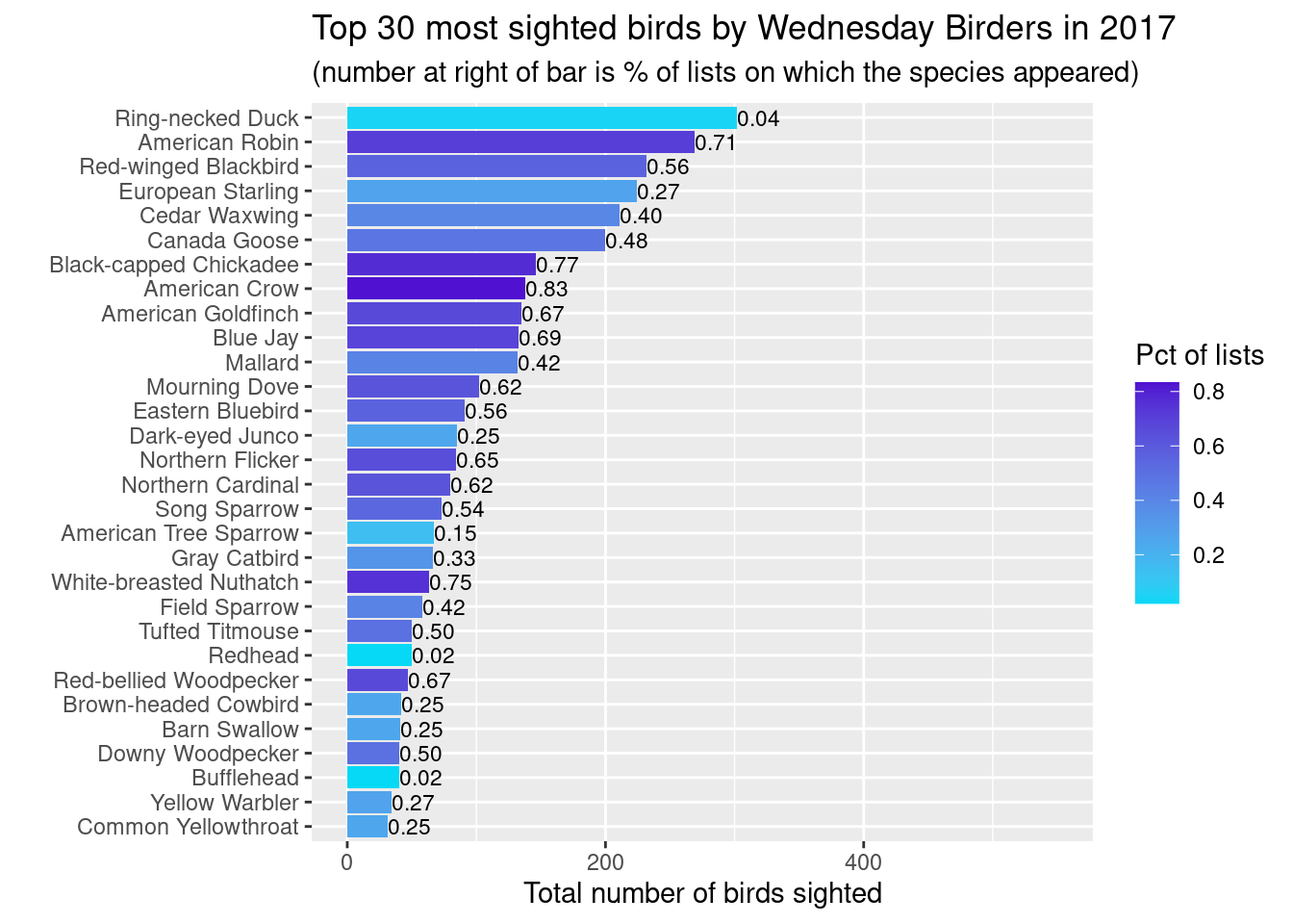
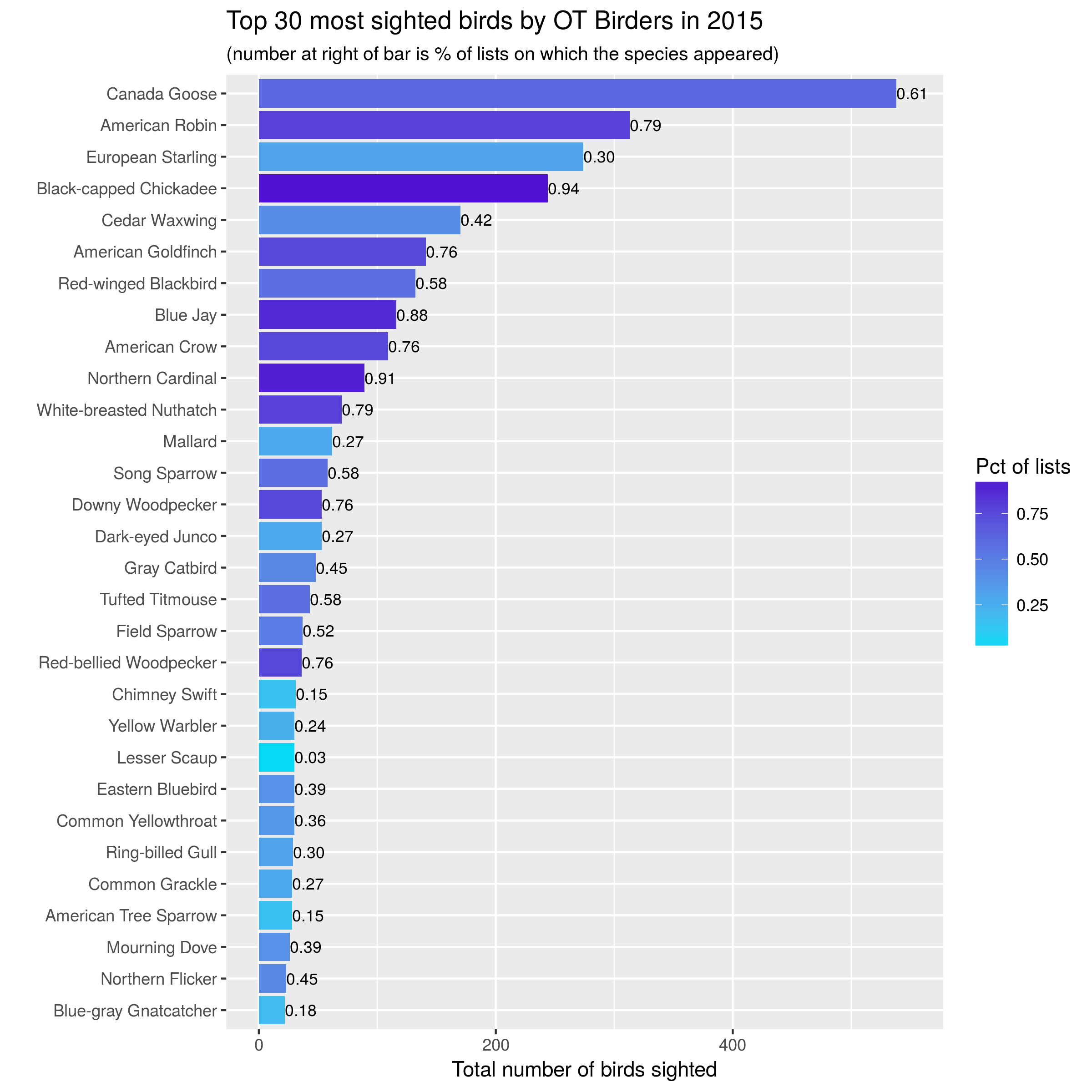
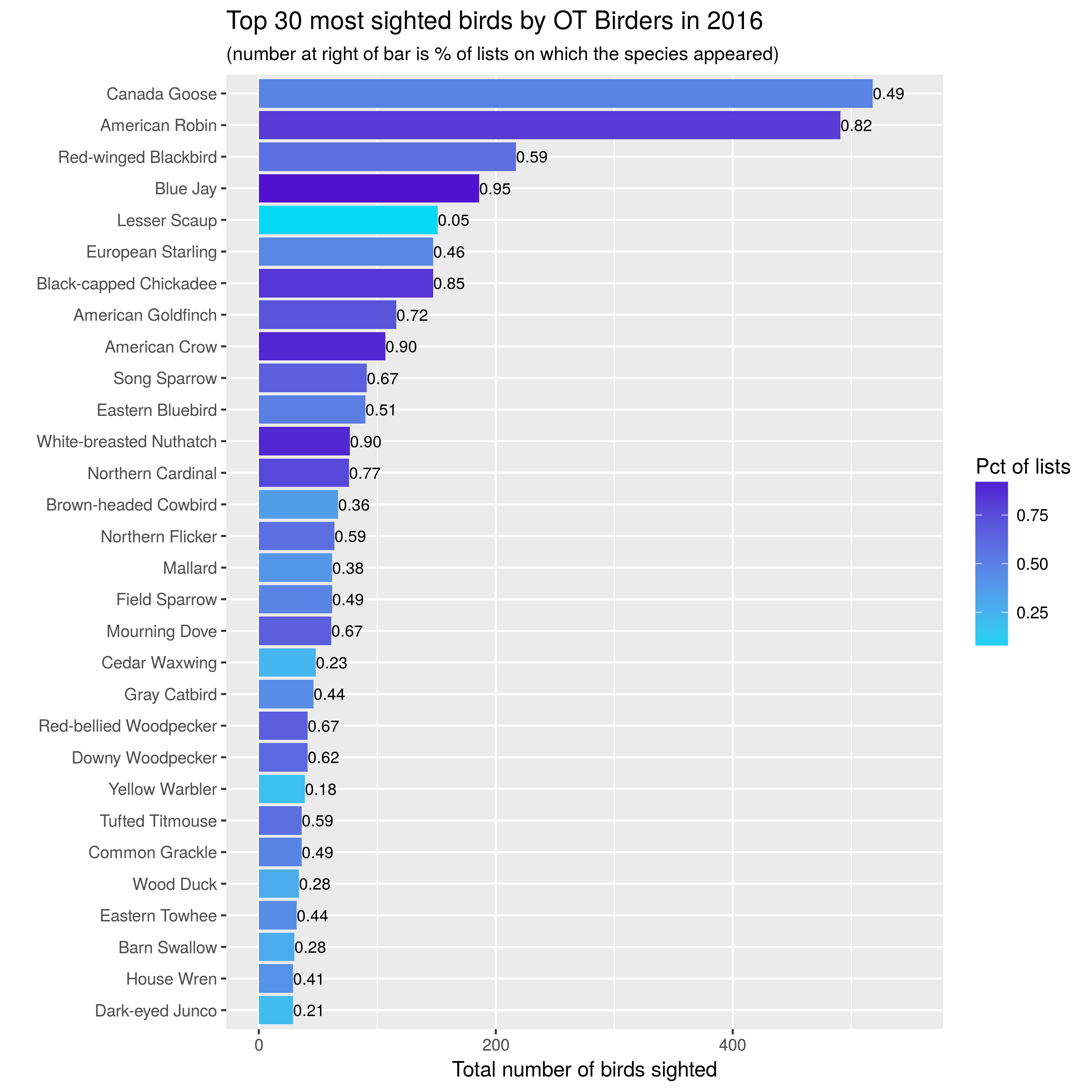
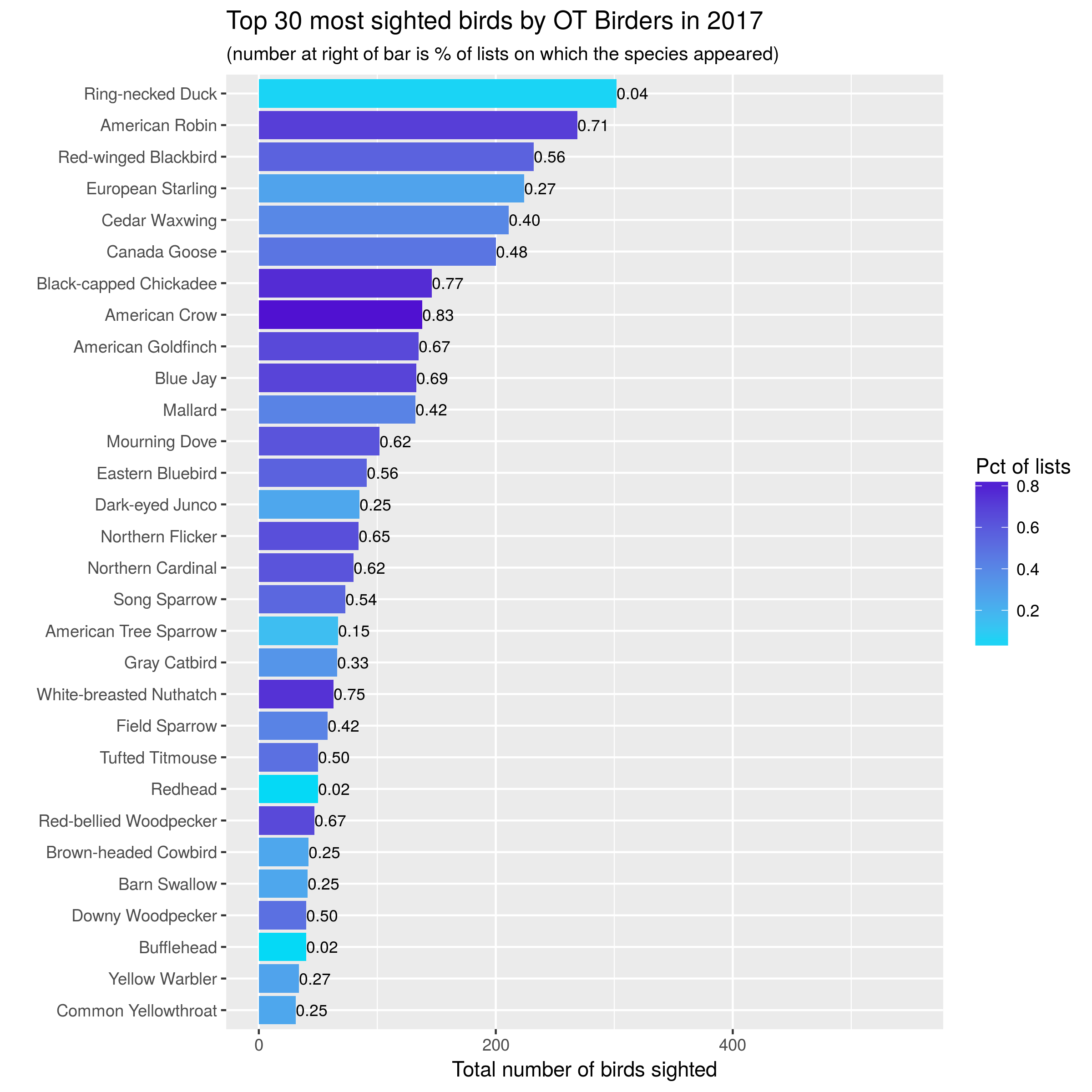
Let’s start with simple bar charts:
one bar per species, one year per graph,
bar length is number of birds seen,
color of bar is related to percentage of lists on which that species seen,
number at end of bar is percentage of lists on which that species seen.
A few observations:
Familiar year round friends such as Canada Goose, American Robin, Black-capped Chicadee, Blue Jay and American Goldfinch are sighted in large numbers and on most outings.
Large flocks of European Starlings lead to them having a high number of sightings but appearing relatively infrequently in our lists. In 2017, one big flock of Ring-necked Ducks gave them the title of most birds seen that year!
The overall composition of the lists are pretty similar across the three years. However, overall numbers appear to be down in 2017. Turns out this is in spite of fact that we had more outings (lists) in 2017 (48) than in 2016 (39). This requires more investigation.
Creating the plots
`summarise()` has regrouped the output.
ℹ Summaries were computed grouped by comName and birding_year.
ℹ Output is grouped by comName.
ℹ Use `summarise(.groups = "drop_last")` to silence this message.
ℹ Use `summarise(.by = c(comName, birding_year))` for per-operation grouping
  (`?dplyr::dplyr_by`) instead.
The plots above are easy to create from a dataframe that looks like this:
The only real trickiness is getting the percentage of lists column computed. We can do it in a few steps using dplyr. For the example below I’ve just hard coded in 2017 as the year of interest. In reality, I embedded the code below in a function and passed the year of interest in.
# Create num species by list dataframenumsp_bylist <- obs_df %>%group_by(year=year(obsDt), obsDt, subId, lastName) %>%count() %>%arrange(year, subId)# Using numsp_bylist, create num lists by datenumlists_bydt <- numsp_bylist %>%group_by(obsDt) %>%summarise(numlists =n() ) %>%filter(numlists >=1) %>%arrange(obsDt)# Usings numlists_bydt, create num lists by yearnumlists_byyear <- numlists_bydt %>%group_by(birding_year=year(obsDt)) %>%summarise(totlists =sum(numlists) )# Now ready to compute species by yearspecies_byyear <- obs_df %>%group_by(comName, birding_year=year(obsDt)) %>%summarize(num_lists =n(),tot_birds =sum(howMany) ) %>%arrange(birding_year, desc(tot_birds))
`summarise()` has regrouped the output.
ℹ Summaries were computed grouped by comName and birding_year.
ℹ Output is grouped by comName.
ℹ Use `summarise(.groups = "drop_last")` to silence this message.
ℹ Use `summarise(.by = c(comName, birding_year))` for per-operation grouping
  (`?dplyr::dplyr_by`) instead.
# Join to numlists_byyear so we can compute pct of lists each species# appeared in.species_byyear <-left_join(species_byyear, numlists_byyear, by ='birding_year') # These would be passed in to function version of this codebird_year <-2017ntop <-30# Compute the percentage of lists on which each species appeardtop_obs_byyear <- species_byyear %>%filter(birding_year == bird_year) %>%mutate(pctlists = num_lists / totlists) %>%arrange(desc(tot_birds)) %>%head(ntop)
Finally we are ready to make the plot. For this post I’m cheating a bit by hard coding in a y-axis limit. In the function version, this can be passed in.
ggplot(top_obs_byyear) +geom_bar(aes(x=reorder(comName, tot_birds), y=tot_birds, fill=pctlists), stat ="identity") +scale_fill_gradient(low='#05D9F6', high='#5011D1') +labs(x="", y="Total number of birds sighted", fill="Pct of lists",title =paste0("Top 30 most sighted birds by Wednesday Birders in ", bird_year),subtitle ="(number at right of bar is % of lists on which the species appeared)") +coord_flip() +geom_text(data=top_obs_byyear,aes(x=reorder(comName,tot_birds),y=tot_birds,label=format(pctlists, digits =1),hjust=0 ), size=3) +ylim(0,550)
Next steps
Now that we’ve got the raw data downloaded and cleaned up, we can do a bunch of exploratory analysis and our Wednesday morning birding group will know a little more about what we’ve been seeing.
 A few observations: