Plotting Great Lakes water level data using R - a 2025 update

They moved the data

Note

This post is an update of a post originally done back in 2018. The location and format for data downloading has changed.

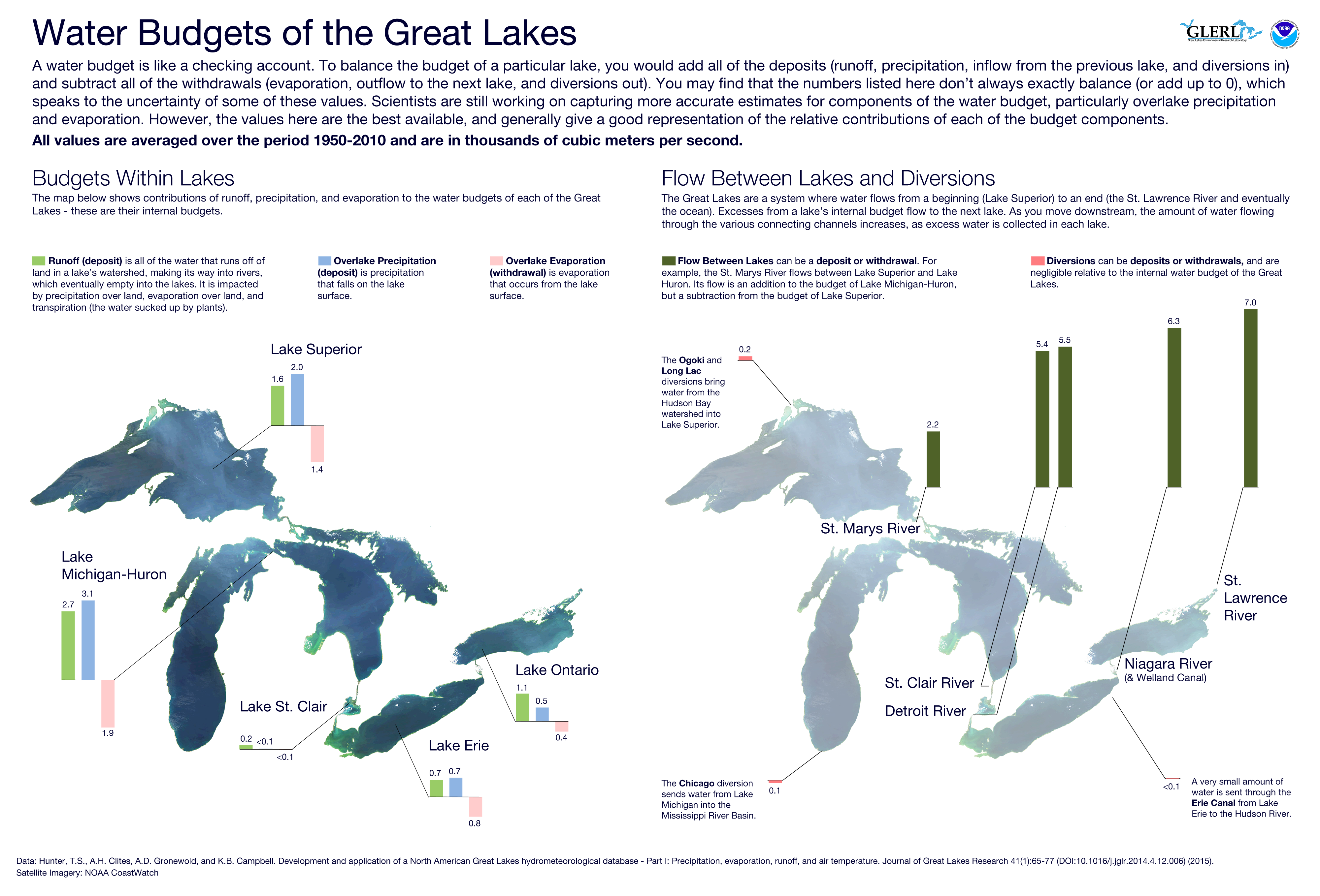
The past few years we have seen record or near record high water levels in all of the Great Lakes. Recently, the levels have dropped. While plots of historical water levels are available on the web, I thought it would be interesting create my own plots using R. In this post I will summarize the steps for using R to:

• download raw historical water level data for the Great Lakes using a few different methods,
• process the raw data to get it into shape for time series plots,
• create time series plots of monthly water levels using ggplot.

Web resources related to Great Lakes water levels

There are a number of good resources for learning about Great Lakes water level monitoring. A few that I’ve found useful as I’ve started to explore this topic include the following. Many of these links have changed since the original 2018 post.

NOAA - Great Lakes Environmental Research Laboratory

• Main - https://www.glerl.noaa.gov/
• Water levels - https://www.glerl.noaa.gov/data/wlevels/
  • tabs for monitoring network, observations and forecasts
• Dashboard - https://www.glerl.noaa.gov/data/wlevels/dashboard/
• Data - https://www.glerl.noaa.gov/data/
• APIs - https://tidesandcurrents.noaa.gov/web_services_info.html
• Water levels and hydrology - https://www.glerl.noaa.gov/data/#hydro
• Tides and Currents - Water levels - https://tidesandcurrents.noaa.gov/water_level_info.html
• Monthly hydrological data - https://www.glerl.noaa.gov/ahps/mnth-hydro.html
• Large Lake Statistical Water Balance Model (L2SWBM) - https://github.com/NOAA-GLERL/L2SWBM
• Great Lakes Seasonal Hydrological Forecasting Products (Experimental) https://www.glerl.noaa.gov/ahps/curfcst.html
• Great Lakes water budget - https://www.glerl.noaa.gov/pubs/brochures/GreatLakesWaterBudgets.png

Other resources

• US Army Corp of Engineers - Great Lakes Information
• Great Lakes Coordination Committee (US and CA)
• Fisheries and Oceans CA - observational data and forecasts

Getting monthly water level data

We will need a few libraries.

library(readr)
library(lubridate)
library(stringr)
library(tidyr)
library(dplyr)
library(ggplot2)

You can download CSV files from NOAA containing monthly water levels for all of the Great Lakes at the following location:

• https://www.lrd.usace.army.mil/Water-Information/Water-Management/Great-Lakes-and-Harbors/Water-Level-Data/

This URL has buttons for downloading long term monthly mean water levels in units desired. The links are:

• https://lre-wm.usace.army.mil/ForecastData/WaterLevelData/GLHYD_data_english.csv
• https://lre-wm.usace.army.mil/ForecastData/WaterLevelData/GLHYD_data_metric.csv

I’ve already downloaded it to a local location to avoid repeated downloads while writing this post.

#data_raw_loc <- "https://lre-wm.usace.army.mil/ForecastData/WaterLevelData/GLHYD_data_metric.csv"
data_raw_loc <- "data_water_level/raw/GLHYD_data_metric.csv"
data_loc <- "data_water_level"

Before reading it into an R dataframe, let’s look at the file format.

# Coordinated Monthly Mean Lakewide Average Water Levels,,,,,,
# Period of record: 1918-2023,,,,,,
"# Units: meters, IGLD 1985",,,,,,
"# Calculated using the coordinated gage network, consisting of:",,,,,,
"# Superior: Marquette and Point Iroquois, MI; Duluth, MN; Michipicoten and Thunder Bay, Ontario",,,,,,
"# Michigan-Huron: Harbor Beach, Mackinaw City and Ludington, MI; Milwaukee, WI; Thessalon and Tobermory, Ontario",,,,,,
"# St. Clair: St. Clair Shores, MI and Belle River, Ontario",,,,,,
"# Erie: Toledo and Cleveland, OH; Port Stanley and Port Colborne, Ontario",,,,,,
"# Ontario: Oswego and Rochester, NY; Cobourg, Port Weller, Toronto, and Kingston, Ontario",,,,,,
#,,,,,,
# Last modified March 2024 Contact: Deanna.C.Fielder@usace.army.mil,,,,,,
#,,,,,,
month,year,Superior,Michigan-Huron,St. Clair,Erie,Ontario
jan,1918,183.25,176.71,174.59,173.9,74.74
feb,1918,183.2,176.73,174.74,173.82,74.72
mar,1918,183.17,176.8,174.74,174.01,74.92
apr,1918,183.14,176.89,174.84,174.02,75.1
may,1918,183.22,176.99,175,173.98,75.09
jun,1918,183.34,177.07,175.14,174.1,75.06
jul,1918,183.4,177.07,175.17,174.12,74.99

A few things to note:

• The top twelve lines are metadata,
• Data goes back to 1918,
• Data is in wide format in that each lake is in its own column.

I used the readr package to read in this csv file. Notice that there is a single column for Lakes Michigan and Huron as they are actually just one big lake that we divide at the Straits of Mackinac - see https://www.glerl.noaa.gov/res/straits/.

mean_lake_level_raw <- read_csv(data_raw_loc, skip = 12)

Data reshaping

In order to facilitate plotting with ggplot2, we are going to need to reshape this data into long format. Each row will be a single monthly reading and there will be a month column and a lake column. Let’s use the tidyr::pivot_longer function.

mean_lake_level_long <- pivot_longer(mean_lake_level_raw, names_to = "lake", values_to = "level_m", cols = 3:7)
rm(mean_lake_level_raw)

Take a peek at the data in long format.

head(mean_lake_level_long)

# A tibble: 6 × 4
  month  year lake           level_m
  <chr> <dbl> <chr>            <dbl>
1 jan    1918 Superior         183. 
2 jan    1918 Michigan-Huron   177. 
3 jan    1918 St. Clair        175. 
4 jan    1918 Erie             174. 
5 jan    1918 Ontario           74.7
6 feb    1918 Superior         183. 

The months are three character strings. Let’s create a date column that we can use for joining the individual tables as well as proper sorting.

mean_lake_level_long$date <- as.POSIXct(str_c(mean_lake_level_long$month, " 1, ",
                                                mean_lake_level_long$year),
                                          format="%b %d, %Y")

mean_lake_level_long <- mean_lake_level_long |> 
  arrange(lake, date)

Check out our work.

head(mean_lake_level_long)

# A tibble: 6 × 5
  month  year lake  level_m date               
  <chr> <dbl> <chr>   <dbl> <dttm>             
1 jan    1918 Erie     174. 1918-01-01 00:00:00
2 feb    1918 Erie     174. 1918-02-01 00:00:00
3 mar    1918 Erie     174. 1918-03-01 00:00:00
4 apr    1918 Erie     174. 1918-04-01 00:00:00
5 may    1918 Erie     174. 1918-05-01 00:00:00
6 jun    1918 Erie     174. 1918-06-01 00:00:00

Alternative data source from GLCC

The Great Lakes Coordination Committee (US and CA) does what it sounds like it does.

The Coordinating Committee on Great Lakes Basic Hydraulic and Hydrologic Data (Coordinating Committee) is a collaboration of the Governments of the United States and Canada for the purpose of agreeing upon the basic hydraulic, hydrologic and vertical control data that is required to manage the Great Lakes and St. Lawrence River.

They also maintain a repository of Great Lakes water level data at https://www.greatlakescc.org/en/coordinating-committee-products-and-datasets/. There are CSV files stored on Google Drive for each lake containing mean monthly water levels since 1918. These are in a different wide format than the data above. Let’s look at the data for Lake Michigan-Huron and compare to the data we just downloaded. Here is what the raw data looks like:

# NAME: LAKE MICHIGAN-HURON MONTHLY MEAN LEVELS 
# UNITS: metres (m) (DATUM: International Great Lakes Datum of 1985) 
# PERIOD OF RECORD: 1918 TO 2024
# DESCRIPTION: Water levels are measured by the National Oceanic and Atmospheric Administration and the  
# Canadian Department of Fisheries and Oceans.  Mean levels are computed as an average
# of a network of gauges and coordinated under the auspices of the Coordinating Committee on 
# Great Lakes Basic Hydraulic and Hydrologic Data      www.greatlakescc.org 
# # All data for the previous 12 months should be considered provisional. 
# note: -9999 means that no data is available for that date 
Year, Jan, Feb, Mar, Apr, May, Jun, Jul, Aug, Sep, Oct, Nov, Dec 
1918,176.71,176.73,176.8,176.89,176.99,177.07,177.07,177.01,176.94,176.83,176.82,176.78 
1919,176.74,176.68,176.68,176.77,176.89,176.92,176.88,176.83,176.72,176.66,176.62,176.55 
1920,176.5,176.47,176.49,176.63,176.68,176.73,176.79,176.76,176.73,176.65,176.57,176.5 
1921,176.44,176.42,176.42,176.54,176.63,176.64,176.6,176.54,176.5,176.44,176.35,176.34 
1922,176.27,176.24,176.28,176.43,176.57,176.63,176.67,176.63,176.56,176.46,176.35,176.25 

A few things to note:

• The top nine lines are metadata,
• Data goes back to 1918,
• Data is in wide format in that each month (instead of lake) is in its own column.

We need to combine the separate lake files and do some reshaping and column manipulation. Again, I’ve already downloaded the five data files to a local folder.

data_cc_raw_loc <-"data_water_level/raw/"

gl_data_raw = list()
gl_data_long = list()

# regex pattern for filename matching
file_pattern <- "\\w+_MonthlyMeanWaterLevels_1918to2024\\.csv$"
gl_files <- list.files(path = data_cc_raw_loc, pattern = file_pattern)

# Loop over the list of matched filenames
for (i in seq_along(gl_files)) {
    filename <- paste0(data_cc_raw_loc, gl_files[i])
    gl_data_raw[[i]] <- read_csv(file = filename, skip = 9)
    # Which lake?
    lake <- str_match(filename, "(Lake\\w+)_Month")[2]
    # Pivot to long format
    gl_data_long[[i]] <- pivot_longer(gl_data_raw[[i]], names_to = "month", values_to = "level_m", cols = 2:13)
    # Add a lake identifier column
    gl_data_long[[i]]$lake <- lake
    # Add date based on month and year
    gl_data_long[[i]]$date <- as.POSIXct(str_c(gl_data_long[[i]]$month, " 1, ",
                                               gl_data_long[[i]]$Year),
                                         format="%b %d, %Y")

}

# Bind all the rows together from the list of dataframes
mean_lake_level_cc_long <- bind_rows(gl_data_long)

# Column renaming and factor seting
mean_lake_level_cc_long <- mean_lake_level_cc_long %>% 
  rename(year = Year)
mean_lake_level_cc_long$lake <- factor(mean_lake_level_cc_long$lake, 
                                       levels = c("LakeSuperior", "LakeMichiganHuron", "LakeStClair", "LakeErie", "LakeOntario"))

This data goes through 2024 whereas the one from the NOAA site hasn’t been updated yet for 2024. Let’s check to see if data is the same through 2023.

level_m_noaa <- mean_lake_level_long %>% 
  select(level_m) 

level_m_cc <- mean_lake_level_cc_long %>% 
  filter(year < 2024) %>% 
  select(level_m)

max_abs_diff <- max(abs(level_m_noaa$level_m - level_m_cc$level_m), na.rm = TRUE)
assertthat::assert_that(max_abs_diff == 0)

[1] TRUE

Confirms that the data is identical from the two sources.

Lake level plotting

If we plot all the lake level time series on one plot, we can see the differences in levels between lakes but the intra-lake variation is hidden by the scale.

ggplot(mean_lake_level_cc_long) + geom_line(aes(x=date, y = level_m, colour = lake)) +
  ylab("Water level (m)")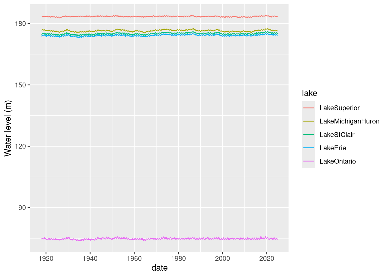

Let’s find the latest month for which we have data and save a version of this dataframe and tag it by the month. Note the use of pull() to convert the the resulting 1x1 dataframe into a value.

last_month_d <- mean_lake_level_cc_long %>% 
  filter(!is.na(level_m)) %>% 
  select(date) %>% 
  summarize(whichmonth = max(date)) %>% 
  pull()

last_month_d

[1] "2024-12-01 EST"

Save as an rds file.

rdsname <- file.path(data_loc, paste0("lake_level_", year(last_month_d), strftime(last_month_d,"%m"), ".rds"))

saveRDS(mean_lake_level_long, rdsname)

Plotting monthly water level data

Let’s compute a bunch of overall historical statistics and include a few as reference lines on the plots. I will use dplyr for the stats.

lake_level_stats <- mean_lake_level_cc_long %>%
  group_by(lake) %>%
  summarize(
    mean_level = mean(level_m, na.rm = TRUE),
    min_level = min(level_m, na.rm = TRUE),
    max_level = max(level_m, na.rm = TRUE),
    p05_level = quantile(level_m, 0.05, na.rm = TRUE),
    p95_level = quantile(level_m, 0.95, na.rm = TRUE),
    sd_level = sd(level_m, na.rm = TRUE),
    cv_level = sd_level / mean_level
  )

lake_level_stats

# A tibble: 5 × 8
  lake      mean_level min_level max_level p05_level p95_level sd_level cv_level
  <fct>          <dbl>     <dbl>     <dbl>     <dbl>     <dbl>    <dbl>    <dbl>
1 LakeSupe…      183.      183.      184.      183.      184.     0.203  0.00110
2 LakeMich…      176.      176.      178.      176.      177.     0.406  0.00230
3 LakeStCl…      175.      174.      176.      174.      176.     0.395  0.00226
4 LakeErie       174.      173.      175.      174.      175.     0.369  0.00212
5 LakeOnta…       74.8      73.7      75.9      74.2      75.3    0.343  0.00459

Let’s try to combine time series with lines from the stats dataframe just created. There are a few approaches to doing this. One way is to add geom_hline objects to the plot. See the following posts for some good ideas on using geom_hline(), adding the reference lines to the legend and controlling their style and color, and controlling the order of plots in a faceted grid.

• https://stackoverflow.com/questions/11846295/how-to-add-different-lines-for-facets
• https://forum.posit.co/t/scale-linetype-manual-not-working/70225
• https://stackoverflow.com/questions/75882636/how-to-specify-geom-hline-color-and-linetype-in-ggplot-legend
• https://stackoverflow.com/questions/75450315/r-facet-grid-order-not-following-levels-with-plotmath

# Create a vector of line style assignments
LINES <- c("mean" = "solid", "5%" = "dotted", "95%" = "dotted")

# Need to explicitly specify order in facet_grid even though levels already set in dataframe
ggplot(mean_lake_level_cc_long, aes(x = date, y = level_m, colour = lake)) +
  facet_grid(factor(lake, levels = c("LakeSuperior", "LakeMichiganHuron", "LakeStClair", "LakeErie", "LakeOntario")) ~ ., scales = "free") +
  geom_hline(data = lake_level_stats, aes(linetype = "mean", yintercept=mean_level)) +
  geom_hline(data = lake_level_stats, aes(linetype = "5%", yintercept=p05_level)) +
  geom_hline(data = lake_level_stats, aes(linetype = "95%", yintercept=p95_level)) +
  geom_line() +
  scale_linetype_manual(values = LINES) +
  ylab("Lake Level (m)") +
  theme(strip.text.y = element_text(size = 16),
        axis.text.x = element_text(size = 14),
        axis.text.y = element_text(size = 10),
        axis.title.x = element_text(size=18),
        axis.title.y = element_text(size=18))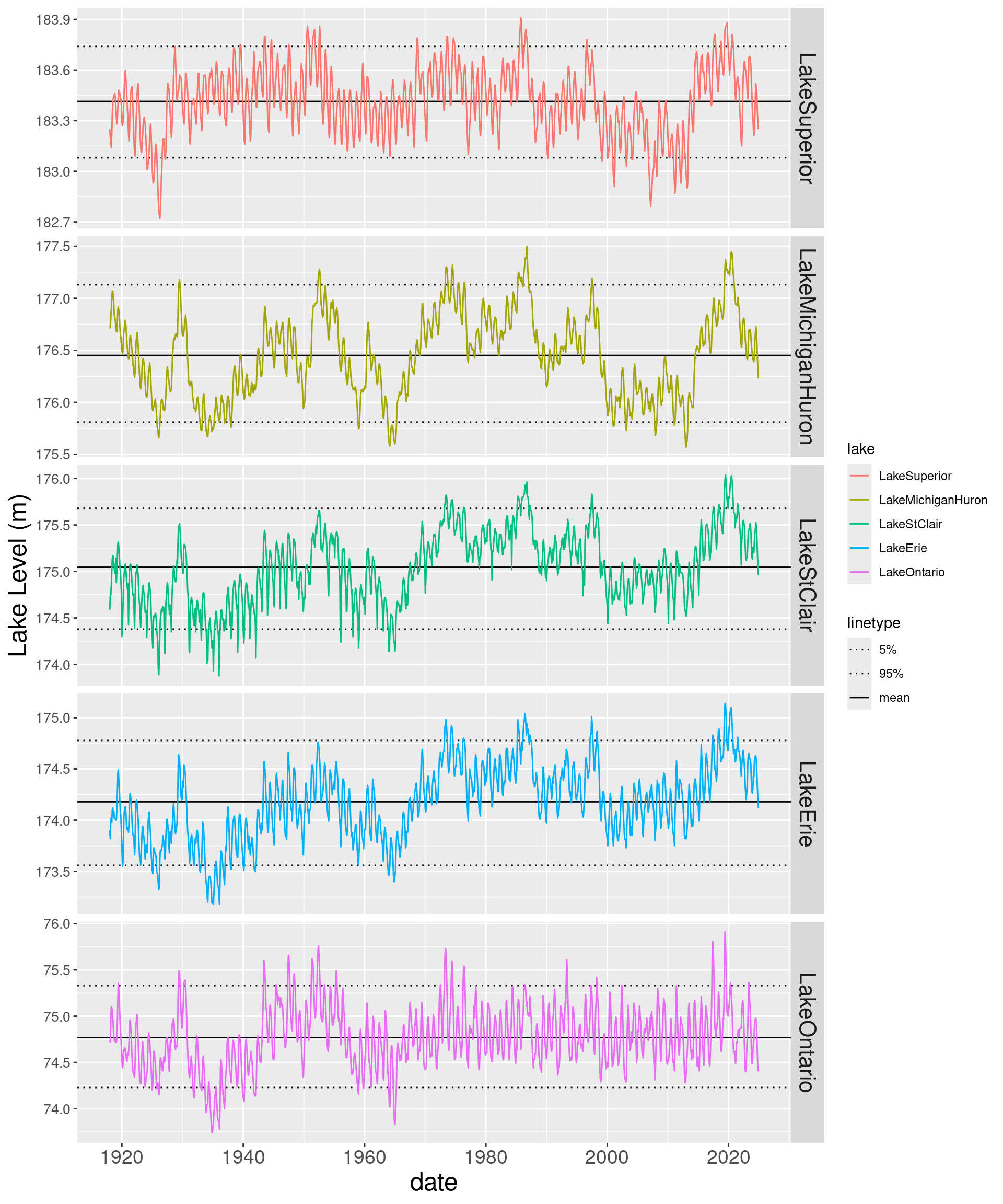

Wow, the lakes are back below their historic (2018 on) mean level. What are the driving factors behind the decrease from the recent peak period?

• less precipitation?
• more evaporation?
• less basin runoff?
• human controls?
• thermal contraction?
• some combination?