pacu <- read.csv('data/pacu.csv')Using R instead of Excel for analyzing recovery room data
Another old-school tutorial on group by analysis with R
R
Note
This post is a bit dated. However, it’s worth keeping around as a look back at the days when the tidyverse was not yet a thing, but tools like ggplot2 and plyr were a sign of things to come.
In my spreadsheet modeling class this semester, I gave an assignment that involved doing some basic pivot tables and histograms for a dataset containing (fake) patient records from a post-anethesia care unit (PACU). It’s the place you go after having surgery until you recover sufficiently to either go home (for outpatient surgery) and head back to your hospital room.
You can find the data, the assignment (PACU_analysis_problem.pdf) and the R Markdown file in my hselab-tutorials github repo. Clone or download a zip.
You’ll see that one of the questions involves having students reflect on why certain kinds of analytical tasks are difficult to do in Excel. I have them read one of my previous posts on using R for a similar analysis task.
So, I thought it would be fun to do some of the things asked for in this Excel assignment but to use R instead. It is a very useful exercise and I think those somewhat new to R (especially coming from an Excel-centric world like a business school) will pick up some good tips and continue to add to their R knowledge base.
Some of the things that this exercise will touch on include: - reading a CSV file and controlling the data types as they come in to an R dataframe - converting Excel date/times to R datetimes (actually to POSIXct) - doing typical date time math - working with R factors, levels and some string parsing - using the plyr package for split-apply-combine analysis (aka “group by” analysis for SQL folks) - avoiding an evil gotcha involving POSIXlt vs POSIXct datetime classes when using plyr
Read the data
We can check out the structure of this dataframe with the str() function. Do a help(str) to learn more about this handy function.
str(pacu)'data.frame': 1688 obs. of 9 variables:
$ VisitNum : int 1 2 3 4 5 6 7 8 9 10 ...
$ Severity : chr "Acuity 1" "Acuity 2" "Acuity 2" "Acuity 2" ...
$ PatType : chr "I" "I" "I" "I" ...
$ RecoveryIn : chr "6/3/2010 19:36" "6/19/2010 9:40" "6/15/2010 0:26" "6/11/2010 13:56" ...
$ RecoveryOut: chr "6/3/2010 19:55" "6/19/2010 12:45" "6/15/2010 1:15" "6/11/2010 15:10" ...
$ RecovMins : int 19 185 49 74 139 79 46 70 29 44 ...
$ DayOfWeek : int 5 7 3 6 3 7 3 6 4 5 ...
$ Hour : int 19 9 0 13 13 11 14 12 9 10 ...
$ Destination: chr "4N" "3N" "4N" "3N" ...Unfortunately, some of our fields weren’t interpreted as we’d like. For example, the date fields RecoveryIn and recovery out were interpreted as factors instead of data. Let’s see if read.csv() has a hook for doing this.
help(read.csv)Hmm, looks like colClasses should do the trick.
pacu <- read.csv('data/pacu.csv',colClasses = c("integer","factor","factor","Date","Date","numeric","factor","factor","factor"))Unfortunately, it butchers the dates.
pacu[1:5,] VisitNum Severity PatType RecoveryIn RecoveryOut RecovMins DayOfWeek Hour
1 1 Acuity 1 I 6-03-20 6-03-20 19 5 19
2 2 Acuity 2 I <NA> <NA> 185 7 9
3 3 Acuity 2 I <NA> <NA> 49 3 0
4 4 Acuity 2 I 6-11-20 6-11-20 74 6 13
5 5 Acuity 2 I 6-08-20 6-08-20 139 3 13
Destination
1 4N
2 3N
3 4N
4 3N
5 3NWorking with dates and times
Let’s read the dates as characters and then convert them using as.Date or strptime function.
pacu <- read.csv('data/pacu.csv',colClasses = c("integer","factor","factor","character","character","numeric","numeric","numeric","factor"))pacu[1:5,] VisitNum Severity PatType RecoveryIn RecoveryOut RecovMins DayOfWeek
1 1 Acuity 1 I 6/3/2010 19:36 6/3/2010 19:55 19 5
2 2 Acuity 2 I 6/19/2010 9:40 6/19/2010 12:45 185 7
3 3 Acuity 2 I 6/15/2010 0:26 6/15/2010 1:15 49 3
4 4 Acuity 2 I 6/11/2010 13:56 6/11/2010 15:10 74 6
5 5 Acuity 2 I 6/8/2010 13:11 6/8/2010 15:30 139 3
Hour Destination
1 19 4N
2 9 3N
3 0 4N
4 13 3N
5 13 3NThe Quick-R site has useful info on the date related functions. http://www.statmethods.net/input/dates.html
Let’s test as.Date and strptime.
as.Date("6/3/2010 19:36",format="%m/%d/%Y %H:%M")[1] "2010-06-03"strptime("6/3/2010 19:36","",format="%m/%d/%Y %H:%M")[1] "2010-06-03 19:36:00 EDT"Hmm, as.Date isn’t displaying the time. A little Googling leads to http://rfunction.com/archives/1912 which confirms we need strptime if we want times. Now, we just need to transform the RecoveryIn and RecoveryOut columns using it.
pacu$RecoveryIn <- strptime(pacu$RecoveryIn,"",format="%m/%d/%Y %H:%M")
pacu$RecoveryOut <- strptime(pacu$RecoveryOut,"",format="%m/%d/%Y %H:%M")
str(pacu)
'data.frame': 1688 obs. of 9 variables:
$ VisitNum : int 1 2 3 4 5 6 7 8 9 10 ...
$ Severity : Factor w/ 5 levels "Acuity 1","Acuity 2",..: 1 2 2 2 2 2 4 2 2 2 ...
$ PatType : Factor w/ 2 levels "I","O": 1 1 1 1 1 1 1 1 1 1 ...
$ RecoveryIn : POSIXlt, format: "2010-06-03 19:36:00" "2010-06-19 09:40:00" ...
$ RecoveryOut: POSIXlt, format: "2010-06-03 19:55:00" "2010-06-19 12:45:00" ...
$ RecovMins : num 19 185 49 74 139 79 46 70 29 44 ...
$ DayOfWeek : num 5 7 3 6 3 7 3 6 4 5 ...
$ Hour : num 19 9 0 13 13 11 14 12 9 10 ...
$ Destination: Factor w/ 7 levels "3N","4N","4S",..: 2 1 2 1 1 2 3 1 2 2 ...POSIXlt is a date-time class. Learn more from Ripley, B. D. and Hornik, K. (2001) Date-time classes. R News, 1/2, 8-11. http://www.r-project.org/doc/Rnews/Rnews_2001-2.pdf.
WARNING: After doing this I carried on and eventually started doing a bunch of analysis with plyr (group by stuff and do counts, sums, means, etc.) When trying to do a group by on two grouping fields I got a strange error. Googling led to the following post in StackOverflow. Hadley Wickham, the creator of plyr chimed in with Use POSIXct dates in data.frames, not POSIXlt. Ok, did that and the weird error went away. The SO post above has some details on the internals of this issue if you are interested. This post on POSIXlt vs POSIXct also sheds light:
First, there’s two internal implementations of date/time: POSIXct, which stores seconds since UNIX epoch (+some other data), and POSIXlt, which stores a list of day, month, year, hour, minute, second, etc. strptime is a function to directly convert character vectors (of a variety of formats) to POSIXlt format. as.POSIXlt converts a variety of data types to POSIXlt. It tries to be intelligent and do the sensible thing - in the case of character, it acts as a wrapper to strptime. as.POSIXct converts a variety of data types to POSIXct. It also tries to be intelligent and do the sensible thing - in the case of character, it runs strptime first, then does the conversion from POSIXlt to POSIXct. It makes sense that strptime is faster, because strptime only handles character input whilst the others try to determine which method to use from input type. It should also be a bit safer in that being handed unexpected data would just give an error, instead of trying to do the intelligent thing that might not be what you want.
The fix is easy.
pacu$RecoveryIn <- as.POSIXct(pacu$RecoveryIn)
pacu$RecoveryOut <- as.POSIXct(pacu$RecoveryOut)
Let’s add a new column called RecoveryMins and which is simply RecoveryOut-RecoveryIn. There is a difftime function that gives us some flexibility in specifying the units (much like DateDiff in the VBA world). However, the default output is a little strange (it’s a “difftime” object) for those used to VBA.
difftime(pacu[1,5],pacu[1,4],"",units="mins")Time difference of 19 minsTo just get a numeric value we can do the following:
as.double(difftime(pacu[1,5],pacu[1,4],"",units="mins"))[1] 19Create the new RecoveryMin column:
pacu$RecoveryMins <- as.double(difftime(pacu$RecoveryOut,pacu$RecoveryIn,"",units="mins"))
head(pacu)
VisitNum Severity PatType RecoveryIn RecoveryOut RecovMins
1 1 Acuity 1 I 2010-06-03 19:36:00 2010-06-03 19:55:00 19
2 2 Acuity 2 I 2010-06-19 09:40:00 2010-06-19 12:45:00 185
3 3 Acuity 2 I 2010-06-15 00:26:00 2010-06-15 01:15:00 49
4 4 Acuity 2 I 2010-06-11 13:56:00 2010-06-11 15:10:00 74
5 5 Acuity 2 I 2010-06-08 13:11:00 2010-06-08 15:30:00 139
6 6 Acuity 2 I 2010-06-05 11:56:00 2010-06-05 13:15:00 79
DayOfWeek Hour Destination RecoveryMins
1 5 19 4N 19
2 7 9 3N 185
3 3 0 4N 49
4 6 13 3N 74
5 3 13 3N 139
6 7 11 4N 79Another requirement in the Excel assignment was to create a few date related, derived, columns: month, day of month, and year. So, a little research reveals that extraction of “date parts” from POSIXlt and POSIXct objects involves using the strftime function and passing a format string. For example, to get the month of RecoveryIn from the first row in the pacu dataframe, we cand do this.
strftime(pacu[1,4],"%Y")[1] "2010"Hmm, we get a character representation. There has to be a better way. There is. There’s a nice little package called lubridate “that makes working with dates fun instead of frustrating”.
# install.packages("lubridate")library(lubridate)
Attaching package: 'lubridate'The following objects are masked from 'package:base':
date, intersect, setdiff, unionA introductory blog post by one of the authors is a good place to start. Also, help(lubridate) is enlightening.
Look how easy it is to parse a date string that’s in a certain format. A POSIXct date-time object is returned.
somedatetime <- mdy_hm("6/3/2010 19:36")
somedatetime
[1] "2010-06-03 19:36:00 UTC"Lubridate has a bunch of easy to remember functions to break apart dates and times in ways that should be quite familiar to MS Office and VBA types.
month(somedatetime)[1] 6mday(somedatetime)[1] 3year(somedatetime)[1] 2010Now we can create new convenience columns to facilitate date related analyses.
pacu$month <- month(pacu$RecoveryIn)
pacu$day <- mday(pacu$RecoveryIn)
pacu$year <- year(pacu$RecoveryIn)
head(pacu)
VisitNum Severity PatType RecoveryIn RecoveryOut RecovMins
1 1 Acuity 1 I 2010-06-03 19:36:00 2010-06-03 19:55:00 19
2 2 Acuity 2 I 2010-06-19 09:40:00 2010-06-19 12:45:00 185
3 3 Acuity 2 I 2010-06-15 00:26:00 2010-06-15 01:15:00 49
4 4 Acuity 2 I 2010-06-11 13:56:00 2010-06-11 15:10:00 74
5 5 Acuity 2 I 2010-06-08 13:11:00 2010-06-08 15:30:00 139
6 6 Acuity 2 I 2010-06-05 11:56:00 2010-06-05 13:15:00 79
DayOfWeek Hour Destination RecoveryMins month day year
1 5 19 4N 19 6 3 2010
2 7 9 3N 185 6 19 2010
3 3 0 4N 49 6 15 2010
4 6 13 3N 74 6 11 2010
5 3 13 3N 139 6 8 2010
6 7 11 4N 79 6 5 2010Factor levels and strings
Let’s also create a new numeric column called Acuity by grabbing the integer off of the end of the Severity values (e.g. “Acuity 1”). This will give us a chance to look at basic string manipulation in R. But first, a trip into the world of factors and levels…
So, R has a substr function that lets you extract substrings from strings. To use it: substr(x, start, stop). It seemed to me that the following should work to pull off the last character in the Severity field for the first row in the pacu dataframe.
substr(pacu[1,2],nchar(pacu[1,2]),nchar(pacu[1,2]))Error in nchar(pacu[1, 2]): 'nchar()' requires a character vectorHuh?
length(pacu[1,2])[1] 1nchar(pacu[1,2])Error in nchar(pacu[1, 2]): 'nchar()' requires a character vectorBut wait, I thought Severity had values like “Acuity 1”? It does, but those are simply levels of the factor (and Severity is a factor). How are factor values stored by R? Start by looking at the numeric conversion of Severity.
# Numeric version of Severity for first 100 rows in pacu
as.numeric(pacu$Severity[1:100])
[1] 1 2 2 2 2 2 4 2 2 2 4 2 2 5 2 4 4 4 2 4 2 2 5 2 2 2 2 2 2 2 2 2 2 2 2 4 2
[38] 2 2 4 2 5 2 2 2 2 3 2 4 2 4 5 4 2 2 4 4 2 4 2 2 2 2 2 2 4 5 2 5 1 5 2 4 2
[75] 4 2 4 4 5 4 1 2 4 2 2 2 4 2 4 5 4 2 5 2 2 2 4 4 1 2What are these integers? They are indices into the levels of the Severity factor. What are the levels?
levels(pacu$Severity)[1] "Acuity 1" "Acuity 2" "Acuity 3" "Acuity 4" "Acuity 5"class(levels(pacu$Severity))[1] "character"The levels themselves are characters. Conveniently, they are also ordered correctly (1-5). We could grab the acuity number a few different ways.
# Let's just test this with the first patient
firstpat <- pacu[1,]

acuity <- as.numeric(firstpat$Severity)
acuity
[1] 1# If we didn't want to rely on them being ordered correctly, we could do some string-fu
sev_string <- levels(firstpat$Severity)[acuity]
acuity_alt <- substr(sev_string,nchar(sev_string),nchar(sev_string))
acuity_alt[1] "1"# Be careful, acuity_alt is a character
acuity_alt <- as.numeric(acuity_alt)
acuity_alt[1] 1Now that we understand how to get the acuity value from the Severity factor, we can make a new column in our data frame.
# Method 1
pacu$acuity <- as.numeric(pacu$Severity)
head(pacu)
VisitNum Severity PatType RecoveryIn RecoveryOut RecovMins
1 1 Acuity 1 I 2010-06-03 19:36:00 2010-06-03 19:55:00 19
2 2 Acuity 2 I 2010-06-19 09:40:00 2010-06-19 12:45:00 185
3 3 Acuity 2 I 2010-06-15 00:26:00 2010-06-15 01:15:00 49
4 4 Acuity 2 I 2010-06-11 13:56:00 2010-06-11 15:10:00 74
5 5 Acuity 2 I 2010-06-08 13:11:00 2010-06-08 15:30:00 139
6 6 Acuity 2 I 2010-06-05 11:56:00 2010-06-05 13:15:00 79
DayOfWeek Hour Destination RecoveryMins month day year acuity
1 5 19 4N 19 6 3 2010 1
2 7 9 3N 185 6 19 2010 2
3 3 0 4N 49 6 15 2010 2
4 6 13 3N 74 6 11 2010 2
5 3 13 3N 139 6 8 2010 2
6 7 11 4N 79 6 5 2010 2# Method 2
pacu$acuity_str <- levels(pacu$Severity)[as.numeric(pacu$Severity)] # Temporary string version
pacu$acuity_alt <- substr(pacu$acuity_str,nchar(pacu$acuity_str),nchar(pacu$acuity_str))
pacu$acuity_str <- NULL # Get rid of the temporary string versionUsing plyr for group by analysis
Load the plyr library to make “group by” (split-apply-combine) analysis easy.
Hadley Wickham (2011). The Split-Apply-Combine Strategy for Data Analysis. Journal of Statistical Software, 40(1), 1-29. http://www.jstatsoft.org/v40/i01/.
library(plyr)Let’s do some basic counts by patient type and acuity.
pivot1 <- ddply(pacu,.(PatType),summarize,numcases = length(VisitNum))
pivot1
PatType numcases
1 I 994
2 O 694pivot2 <- ddply(pacu,.(acuity),summarize,numcases = length(VisitNum))
pivot2 acuity numcases
1 1 160
2 2 1072
3 3 111
4 4 263
5 5 82pivot3 <- ddply(pacu,.(PatType,acuity),summarize,numcases = length(VisitNum))
pivot3 PatType acuity numcases
1 I 1 53
2 I 2 563
3 I 3 56
4 I 4 243
5 I 5 79
6 O 1 107
7 O 2 509
8 O 3 55
9 O 4 20
10 O 5 3Want to view it more like a 2-D Excel pivot table? This is a job for another useful Hadley Wickham package - reshape2.
Reshape lets you flexibly restructure and aggregate data using just two functions: melt and cast.
library(reshape2)Here’s a good introductory tutorial on reshape2. It covers the notion of wide and long data formats and using melt and cast to move between these two formats.
Let’s cast pivot3 so that acuity swings up from the rows and into the column headers. The “pivot table” will get wider.
dcast(pivot3,PatType ~ acuity,value.var = "numcases") PatType 1 2 3 4 5
1 I 53 563 56 243 79
2 O 107 509 55 20 3Same idea applied to counting cases by hour of day and acuity…
pivot4 <- ddply(pacu,.(acuity,Hour),summarize,numcases = length(VisitNum))
pivot4
acuity Hour numcases
1 1 2 1
2 1 8 14
3 1 9 14
4 1 10 16
5 1 11 17
6 1 12 18
7 1 13 16
8 1 14 15
9 1 15 5
10 1 16 7
11 1 17 10
12 1 18 5
13 1 19 9
14 1 20 3
15 1 21 6
16 1 22 4
17 2 0 10
18 2 2 4
19 2 3 5
20 2 4 3
21 2 5 5
22 2 6 3
23 2 7 2
24 2 8 63
25 2 9 100
26 2 10 123
27 2 11 119
28 2 12 94
29 2 13 104
30 2 14 89
31 2 15 93
32 2 16 68
33 2 17 57
34 2 18 42
35 2 19 32
36 2 20 20
37 2 21 14
38 2 22 13
39 2 23 9
40 3 0 1
41 3 1 3
42 3 3 1
43 3 5 1
44 3 6 2
45 3 7 1
46 3 8 4
47 3 9 15
48 3 10 15
49 3 11 7
50 3 12 8
51 3 13 8
52 3 14 11
53 3 15 8
54 3 16 7
55 3 17 4
56 3 18 2
57 3 19 4
58 3 20 5
59 3 22 3
60 3 23 1
61 4 1 2
62 4 2 2
63 4 3 2
64 4 8 3
65 4 9 16
66 4 10 19
67 4 11 25
68 4 12 24
69 4 13 29
70 4 14 29
71 4 15 28
72 4 16 31
73 4 17 17
74 4 18 13
75 4 19 8
76 4 20 6
77 4 21 5
78 4 22 1
79 4 23 3
80 5 0 1
81 5 4 1
82 5 6 1
83 5 9 2
84 5 10 9
85 5 11 6
86 5 12 7
87 5 13 10
88 5 14 4
89 5 15 14
90 5 16 3
91 5 17 6
92 5 18 7
93 5 19 5
94 5 21 5
95 5 23 1dcast(pivot4,acuity ~ Hour,value.var = "numcases",fill=0) acuity 0 1 2 3 4 5 6 7 8 9 10 11 12 13 14 15 16 17 18 19 20 21 22 23
1 1 0 0 1 0 0 0 0 0 14 14 16 17 18 16 15 5 7 10 5 9 3 6 4 0
2 2 10 0 4 5 3 5 3 2 63 100 123 119 94 104 89 93 68 57 42 32 20 14 13 9
3 3 1 3 0 1 0 1 2 1 4 15 15 7 8 8 11 8 7 4 2 4 5 0 3 1
4 4 0 2 2 2 0 0 0 0 3 16 19 25 24 29 29 28 31 17 13 8 6 5 1 3
5 5 1 0 0 0 1 0 1 0 0 2 9 6 7 10 4 14 3 6 7 5 0 5 0 1# Flip the axes
pivot5 <- ddply(pacu,.(Hour,acuity),summarize,numcases = length(VisitNum))
pivot5 Hour acuity numcases
1 0 2 10
2 0 3 1
3 0 5 1
4 1 3 3
5 1 4 2
6 2 1 1
7 2 2 4
8 2 4 2
9 3 2 5
10 3 3 1
11 3 4 2
12 4 2 3
13 4 5 1
14 5 2 5
15 5 3 1
16 6 2 3
17 6 3 2
18 6 5 1
19 7 2 2
20 7 3 1
21 8 1 14
22 8 2 63
23 8 3 4
24 8 4 3
25 9 1 14
26 9 2 100
27 9 3 15
28 9 4 16
29 9 5 2
30 10 1 16
31 10 2 123
32 10 3 15
33 10 4 19
34 10 5 9
35 11 1 17
36 11 2 119
37 11 3 7
38 11 4 25
39 11 5 6
40 12 1 18
41 12 2 94
42 12 3 8
43 12 4 24
44 12 5 7
45 13 1 16
46 13 2 104
47 13 3 8
48 13 4 29
49 13 5 10
50 14 1 15
51 14 2 89
52 14 3 11
53 14 4 29
54 14 5 4
55 15 1 5
56 15 2 93
57 15 3 8
58 15 4 28
59 15 5 14
60 16 1 7
61 16 2 68
62 16 3 7
63 16 4 31
64 16 5 3
65 17 1 10
66 17 2 57
67 17 3 4
68 17 4 17
69 17 5 6
70 18 1 5
71 18 2 42
72 18 3 2
73 18 4 13
74 18 5 7
75 19 1 9
76 19 2 32
77 19 3 4
78 19 4 8
79 19 5 5
80 20 1 3
81 20 2 20
82 20 3 5
83 20 4 6
84 21 1 6
85 21 2 14
86 21 4 5
87 21 5 5
88 22 1 4
89 22 2 13
90 22 3 3
91 22 4 1
92 23 2 9
93 23 3 1
94 23 4 3
95 23 5 1dcast(pivot5,Hour ~ acuity,value.var = "numcases",fill=0) Hour 1 2 3 4 5
1 0 0 10 1 0 1
2 1 0 0 3 2 0
3 2 1 4 0 2 0
4 3 0 5 1 2 0
5 4 0 3 0 0 1
6 5 0 5 1 0 0
7 6 0 3 2 0 1
8 7 0 2 1 0 0
9 8 14 63 4 3 0
10 9 14 100 15 16 2
11 10 16 123 15 19 9
12 11 17 119 7 25 6
13 12 18 94 8 24 7
14 13 16 104 8 29 10
15 14 15 89 11 29 4
16 15 5 93 8 28 14
17 16 7 68 7 31 3
18 17 10 57 4 17 6
19 18 5 42 2 13 7
20 19 9 32 4 8 5
21 20 3 20 5 6 0
22 21 6 14 0 5 5
23 22 4 13 3 1 0
24 23 0 9 1 3 1Histograms, box plots and percentiles of recovery time
Now let’s look at some histograms of recovery time.
library(ggplot2)# Basic histogram for ScheduledDaysInAdvance. Each bin is 4 wide.
ggplot(pacu, aes(x=RecoveryMins)) + geom_histogram(binwidth=20)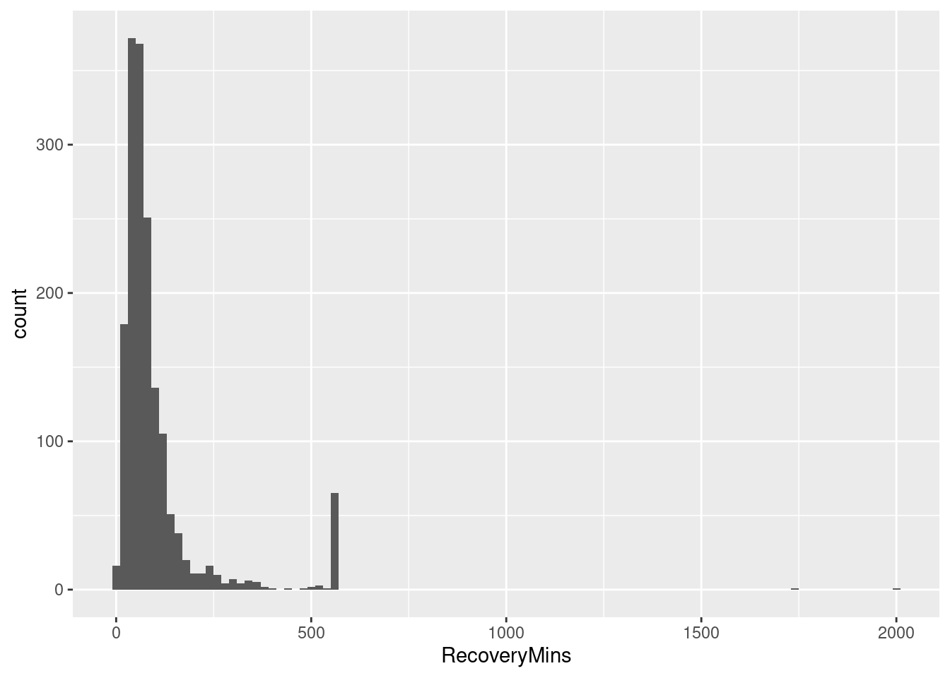
Hmm, that spike in the right tail raises some questions about the data. We’ll ignore for now.
While there are a number of ways to create histograms in Excel (Data Analysis Tool-Pak, FREQUENCY() array function, pivot table with grouped row field), it’s a tedious pain to do them by some factor like acuity. In general, “small multiples” are no fun at all in Excel. In R, it’s easy.
# Histogram with frequencies
ggplot(pacu, aes(x = RecoveryMins)) + facet_wrap(~Severity) + geom_histogram(aes(y = ..density..),binwidth = 10) +
  coord_cartesian(xlim = c(0, 500))
Warning: The dot-dot notation (`..density..`) was deprecated in ggplot2 3.4.0.
ℹ Please use `after_stat(density)` instead.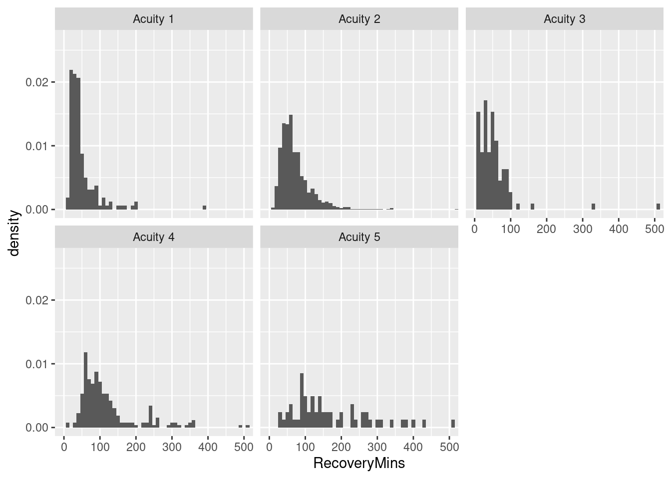
Box plots anyone?
ggplot(pacu, aes(x = Severity, y = RecoveryMins)) + geom_boxplot()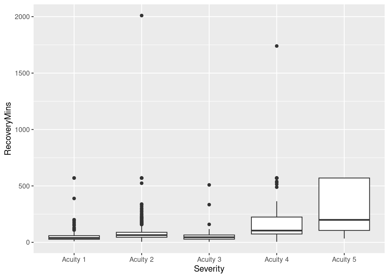
ggplot(pacu, aes(x = Severity, y = RecoveryMins)) + geom_boxplot() + coord_cartesian(ylim = c(0, 750))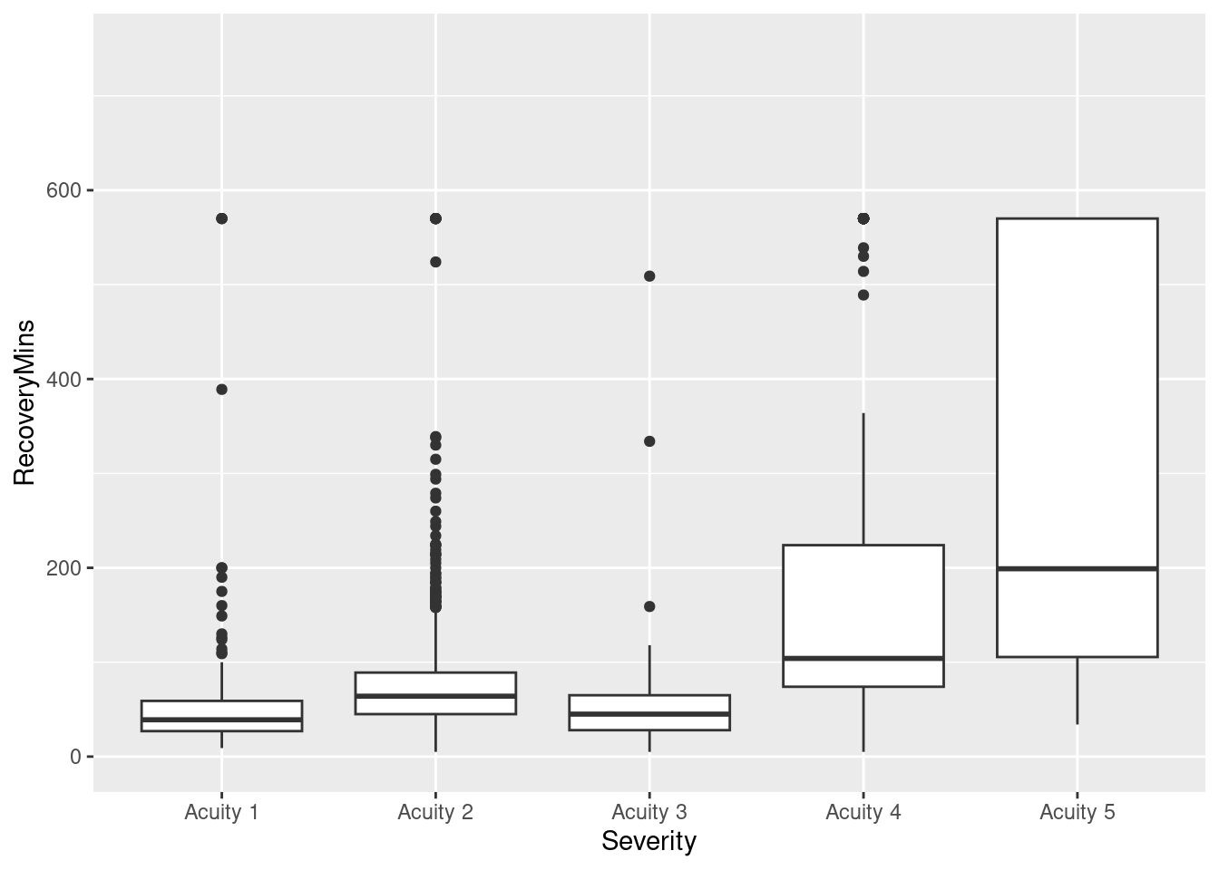
Similarly, percentiles by factor levels is hideous in Excel and easy in R.
pivot6 <- ddply(pacu,.(PatType,acuity),summarize,p95 = quantile(RecoveryMins,0.95))
dcast(pivot6,PatType ~ acuity,value.var = "p95")
PatType 1 2 3 4 5
1 I 461.4 179 108.25 570 570.0
2 O 107.0 144 91.20 301 154.5Now, the rest of the assignment asks the student to construct an Excel based “dashboard” which combines various relevant visualizations of PACU statistics for the PACU manager. Alternatively, one could use a tool like Tableau to create compelling data visualizations. Now, how might one use R to do something like these dashboards? A task for another day.