library(auk)
library(dplyr)
library(ggplot2)
library(lubridate)Create an eBird DuckDB database for use with R
Dealing with large eBird files in R
r
ebird
birding
database
dplyr
The challenge
There is a large amount of data available in the eBird database based on user submitted eBird checklists. Any eBird user can apply for access and download all or a subset of the data as tab delimited text files. One file contains what is known as the eBird Basic Data (EBD) and the other contains Sampling Event Data (SED). For the EBD, each row is an individual species observation on an individual eBird checklist. The SED file contains one row per checklist. There is well over 100Gb of data available representing hundreds of millions of checklists submitted from around the world. A Custom Download page makes it easy to select a subset of the data for download based on a given species, region, or time period.
Before attempting to load eBird data into R dataframes for analysis, I worked through the extremely informative Best Practices for Using eBird Data guide. If you haven’t already, you should do this before attempting the kind of thing described in this blog post.
It’s not terribly difficult to bump up against memory (RAM) limits if you get a little over eager and try to load a large eBird dataset into an R dataframe. Thankfully, there are various ways to use R for analysis on data that resides in an external database. That’s what this post is all about. I decided to try out the newish DuckDB database which can be used with R and which bills itself as a “fast, in-process, analytical database”. Seems perfect for analyzing large eBird datasets.
However, creating and populating a DuckDB database for a large eBird data download can be challenging. The main tool for working with downloaded eBird data is the R library, auk. In addition to facilitating filtering eBird data, the auk package is used for several important data preparation steps. Since R wants to load data entirely into memory, large datasets can be problematic. In this post we will show how you can load eBird data into a DuckDB database to facilitate analysis of large eBird data files. Along the way we will learn about various other challenges associated with eBird data.
The first analysis task
Let’s start by analyzing a small amount of eBird data using R. We will:
- use
aukto create small text files of observations and checklists, - use
auk::read_edb()andauk::read_sampling()to read the text files into R dataframes, - create an empty database and load the R dataframes into database tables using the
duckdb,dbplyrandDBIpackages, - run some basic
dplyrqueries on the observation and sampling event data.
After that, we’ll explore the challenges that arise when the eBird text files are not small and show how we can load large datasets into a DuckDB database and query it with dplyr or duckplyr (a “drop-in” replacement for dplyr).
For this part we will need the following libraries.
Filtering eBird data with auk
The auk: eBird Data Extraction and Processing in R package makes it easy to create and apply text filters to eBird data to create smaller datasets that can comfortably be analyzed in R. Under the hood, auk uses AWK, the widely available Linux/Mac utility (available for Windows via Cygwin) for text file processing. The output of the filtering step are just text files - one for observations and one for sampling events. These text files are formatted exactly like the original text files downloaded from eBird.
auk makes it easy to filter by various criterion:
- species,
- observation date,
- region (country, state, BCR, bounding box),
- time of day,
- effort (duration, distance),
- specific projects (e.g. breeding bird survey),
- protocol (e.g. traveling),
- complete checklist status.
On June 19, 2024 I submitted a request for all of the eBird data for the state of Michigan. On the 15th of each month, the previous month’s data becomes available. So, I would get data through May of 2024. The next day I received an email from eBird with a link to a compressed archive containing the raw data as well as various metadata files.
ls -l data/ebd_US-MI_smp_relMay-2024/total 12673100
-rw-rw-r-- 1 mark mark 1960 Jun 18 13:09 BCRCodes.txt
-rw-rw-r-- 1 mark mark 632528 Jun 18 13:09 BirdLifeKBACodes.txt
-rw-rw-r-- 1 mark mark 654510629 Jun 18 13:06 ebd_US-MI_smp_relMay-2024_sampling.txt
-rw-rw-r-- 1 mark mark 12321474745 Jun 18 10:25 ebd_US-MI_smp_relMay-2024.txt
-rw-rw-r-- 1 mark mark 431439 Jun 18 13:09 eBird_Basic_Dataset_Metadata_v1.15.pdf
-rw-rw-r-- 1 mark mark 126957 Jun 18 13:09 IBACodes.txt
-rw-rw-r-- 1 mark mark 103 Jun 18 13:09 recommended_citation.txt
-rw-rw-r-- 1 mark mark 6703 Jun 18 13:09 terms_of_use.txt
-rw-rw-r-- 1 mark mark 39670 Jun 18 13:09 USFWSCodes.txtThe ebd_US-MI_smp_relMay-2024.txt file is a little over 12.3Gb and contains the EBD data. We’ll refer to these as the observations. The ebd_US-MI_smp_relMay-2024_sampling.txt file contains the SED data - these are the sampling events. The sampling event file is smaller as it contains one row per checklist whereas the observations include, for each checklist, a row with information relating to every species observed. Clearly, we are not going to be attempting to load a 12.3Gb file into an R dataframe.
We’ll start by using auk to filter the data to create a small sample dataset for exploration.
# Set the filenames for the checklist and sample data
f_ebd <- 'data/ebd_US-MI_smp_relMay-2024/ebd_US-MI_smp_relMay-2024.txt'
f_smp <- 'data/ebd_US-MI_smp_relMay-2024/ebd_US-MI_smp_relMay-2024_sampling.txt'
Next we create an auk_ebd object. This object does not contain the raw data. It’s just an object for storing pointers to our data files and various filters we might add later.
ebdsmp <- auk_ebd(f_ebd, file_sampling = f_smp)Let’s start by looking at one day of data to avoid problems related to giant dataframes. If you’ve used auk before, the following two items will be familiar to you. If not, don’t worry about it as we’ll discuss them later.
- we will not collapse the observation and sampling event data into a single dataframe as this will greatly reduce the data storage requirements,
- we will not use
auk_zerofill()either as we aren’t interested right now in absence data and this will keep the file size smaller.
rerun <- FALSE

# Specify output filenames for the filtered data
file_ebd <- "data/ebd_20240519_MI.txt"
file_smp <- "data/smp_20240519_MI.txt"

if (rerun) {
  list_year <- 2024
  ebdsmp %>%
    # date: use standard ISO date format `"YYYY-MM-DD"` with * for wildcard
    auk_date(date = c(paste0(list_year,"-05-19"), paste0(list_year,"-05-19"))) %>%
    # complete: all species seen or heard are recorded (this field is in ebd)
    auk_complete() %>%
    auk_filter(file = file_ebd, file_sampling = file_smp, overwrite = TRUE)
}
In our case, we have downloaded all of the eBird data for the state of Michigan. Our filtering step just ensures we are only working with complete checklists and the filtered text files are still over 11Gb. Specifically:
- this data is NOT zero filled,
- this data has NOT had shared checklists collapsed,
- this data has NOT had taxonomy rollup done.
Reading filtered text files into R dataframes
Now we can use auk::read_ebd() and auk::read_sampling()
observations_df <- read_ebd(file_ebd, unique = TRUE)
sampling_events_df <- read_sampling(file_smp, unique = TRUE)
How big are the two dataframes?
nrow(observations_df)[1] 31100nrow(sampling_events_df)[1] 1451The column names have been cleaned up and some data types changed.
str(observations_df)tibble [31,100 × 48] (S3: tbl_df/tbl/data.frame)
$ checklist_id : chr [1:31100] "G12405482" "G12405614" "G12405614" "G12405614" ...
$ global_unique_identifier : chr [1:31100] "URN:CornellLabOfOrnithology:EBIRD:OBS2171548530" "URN:CornellLabOfOrnithology:EBIRD:OBS2171639660" "URN:CornellLabOfOrnithology:EBIRD:OBS2171639653" "URN:CornellLabOfOrnithology:EBIRD:OBS2171639654" ...
$ last_edited_date : chr [1:31100] "2024-05-20 12:33:05.670199" "2024-05-19 06:00:38.809563" "2024-05-19 06:00:38.809563" "2024-05-19 06:00:38.809563" ...
$ taxonomic_order : num [1:31100] 9011 33252 324 21168 6479 ...
$ category : chr [1:31100] "species" "species" "species" "species" ...
$ taxon_concept_id : chr [1:31100] "avibase-BDBB04D5" "avibase-730AC20E" "avibase-B59E1863" "avibase-69544B59" ...
$ common_name : chr [1:31100] "Barred Owl" "Red-winged Blackbird" "Canada Goose" "American Crow" ...
$ scientific_name : chr [1:31100] "Strix varia" "Agelaius phoeniceus" "Branta canadensis" "Corvus brachyrhynchos" ...
$ exotic_code : chr [1:31100] NA NA NA NA ...
$ observation_count : chr [1:31100] "3" "1" "13" "1" ...
$ breeding_code : chr [1:31100] NA NA NA NA ...
$ breeding_category : chr [1:31100] NA NA NA NA ...
$ behavior_code : chr [1:31100] NA NA NA NA ...
$ age_sex : chr [1:31100] NA NA NA NA ...
$ country : chr [1:31100] "United States" "United States" "United States" "United States" ...
$ country_code : chr [1:31100] "US" "US" "US" "US" ...
$ state : chr [1:31100] "Michigan" "Michigan" "Michigan" "Michigan" ...
$ state_code : chr [1:31100] "US-MI" "US-MI" "US-MI" "US-MI" ...
$ county : chr [1:31100] "Gladwin" "Iosco" "Iosco" "Iosco" ...
$ county_code : chr [1:31100] "US-MI-051" "US-MI-069" "US-MI-069" "US-MI-069" ...
$ iba_code : chr [1:31100] "US-MI_3775" "US-MI_3811" "US-MI_3811" "US-MI_3811" ...
$ bcr_code : int [1:31100] 12 NA NA NA NA NA NA NA NA NA ...
$ usfws_code : chr [1:31100] NA NA NA NA ...
$ atlas_block : chr [1:31100] NA NA NA NA ...
$ locality : chr [1:31100] "Molasses River Retreat" "Tawas Bay" "Tawas Bay" "Tawas Bay" ...
$ locality_id : chr [1:31100] "L26321465" "L1843221" "L1843221" "L1843221" ...
$ locality_type : chr [1:31100] "P" "H" "H" "H" ...
$ latitude : num [1:31100] 43.9 44.3 44.3 44.3 44.3 ...
$ longitude : num [1:31100] -84.3 -83.5 -83.5 -83.5 -83.5 ...
$ observation_date : Date[1:31100], format: "2024-05-19" "2024-05-19" ...
$ time_observations_started: chr [1:31100] "04:47:00" "05:54:00" "05:54:00" "05:54:00" ...
$ observer_id : chr [1:31100] "obsr1077102,obsr502473" "obsr167561,obsr273509" "obsr167561,obsr273509" "obsr167561,obsr273509" ...
$ sampling_event_identifier: chr [1:31100] "S175525573,S175525574" "S175533693,S175533694" "S175533693,S175533694" "S175533693,S175533694" ...
$ protocol_type : chr [1:31100] "Stationary" "Traveling" "Traveling" "Traveling" ...
$ protocol_code : chr [1:31100] "P21" "P22" "P22" "P22" ...
$ project_code : chr [1:31100] "EBIRD" "EBIRD" "EBIRD" "EBIRD" ...
$ duration_minutes : int [1:31100] 6 4 4 4 4 4 4 4 4 4 ...
$ effort_distance_km : num [1:31100] NA 2.72 2.72 2.72 2.72 2.72 2.72 2.72 2.72 2.72 ...
$ effort_area_ha : num [1:31100] NA NA NA NA NA NA NA NA NA NA ...
$ number_observers : int [1:31100] 2 2 2 2 2 2 2 2 2 2 ...
$ all_species_reported : logi [1:31100] TRUE TRUE TRUE TRUE TRUE TRUE ...
$ group_identifier : chr [1:31100] "G12405482" "G12405614" "G12405614" "G12405614" ...
$ has_media : logi [1:31100] TRUE FALSE FALSE FALSE FALSE FALSE ...
$ approved : logi [1:31100] TRUE TRUE TRUE TRUE TRUE TRUE ...
$ reviewed : logi [1:31100] FALSE FALSE FALSE FALSE FALSE FALSE ...
$ reason : chr [1:31100] NA NA NA NA ...
$ trip_comments : chr [1:31100] NA NA NA NA ...
$ species_comments : chr [1:31100] NA NA NA NA ...
- attr(*, "rollup")= logi TRUEThe observation_count filed has a character data type, likely due to the ‘X’ values that are valid user inputs.
observations_df %>%
  filter(observation_count == 'X') %>%
  group_by(observation_count) %>%
  count()
# A tibble: 1 × 2
# Groups: observation_count [1]
observation_count n
<chr> <int>
1 X 820Change it to integer so that we can do math with it. The ‘X’ values will become NA and we’ll have to be careful with it if doing math on observation_count.
# Change observation_count to integer
observations_df$observation_count <- as.integer(observations_df$observation_count)
Warning: NAs introduced by coercionstr(sampling_events_df)tibble [1,451 × 31] (S3: tbl_df/tbl/data.frame)
$ checklist_id : chr [1:1451] "S176512162" "S175546547" "S179823549" "S179822252" ...
$ last_edited_date : chr [1:1451] "2024-05-23 08:03:00.886549" "2024-05-19 07:24:04.965131" "2024-06-06 21:01:29.107477" "2024-06-06 20:49:48.256139" ...
$ country : chr [1:1451] "United States" "United States" "United States" "United States" ...
$ country_code : chr [1:1451] "US" "US" "US" "US" ...
$ state : chr [1:1451] "Michigan" "Michigan" "Michigan" "Michigan" ...
$ state_code : chr [1:1451] "US-MI" "US-MI" "US-MI" "US-MI" ...
$ county : chr [1:1451] "Manistee" "Iosco" "Huron" "Huron" ...
$ county_code : chr [1:1451] "US-MI-101" "US-MI-069" "US-MI-063" "US-MI-063" ...
$ iba_code : chr [1:1451] NA NA NA NA ...
$ bcr_code : int [1:1451] 12 12 NA NA 12 23 23 12 12 22 ...
$ usfws_code : chr [1:1451] NA NA NA NA ...
$ atlas_block : chr [1:1451] NA NA NA NA ...
$ locality : chr [1:1451] "Arcadia Dunes Grasslands" "Sanctuary, Wilber Township, Iosco County" "Harbor Beach (general)" "Harbor Beach (general)" ...
$ locality_id : chr [1:1451] "L1000010" "L1000261" "L1002678" "L1002678" ...
$ locality_type : chr [1:1451] "H" "P" "H" "H" ...
$ latitude : num [1:1451] 44.5 44.4 43.8 43.8 47.4 ...
$ longitude : num [1:1451] -86.2 -83.5 -82.6 -82.6 -88 ...
$ observation_date : Date[1:1451], format: "2024-05-19" "2024-05-19" ...
$ time_observations_started: chr [1:1451] "11:00:00" "06:06:00" "16:15:00" "14:00:00" ...
$ observer_id : chr [1:1451] "obsr2398384" "obsr114260" "obsr201518" "obsr201518" ...
$ sampling_event_identifier: chr [1:1451] "S176512162" "S175546547" "S179823549" "S179822252" ...
$ protocol_type : chr [1:1451] "Traveling" "Traveling" "Traveling" "Traveling" ...
$ protocol_code : chr [1:1451] "P22" "P22" "P22" "P22" ...
$ project_code : chr [1:1451] "EBIRD" "EBIRD" "EBIRD" "EBIRD" ...
$ duration_minutes : int [1:1451] 120 59 20 30 27 30 140 240 5 20 ...
$ effort_distance_km : num [1:1451] 19.312 0.647 4.828 6.437 0.833 ...
$ effort_area_ha : num [1:1451] NA NA NA NA NA NA NA NA NA NA ...
$ number_observers : int [1:1451] 2 1 1 1 1 1 1 2 1 1 ...
$ all_species_reported : logi [1:1451] TRUE TRUE TRUE TRUE TRUE TRUE ...
$ group_identifier : chr [1:1451] NA NA NA NA ...
$ trip_comments : chr [1:1451] NA "Sunny, 69-61 F" NA NA ...
- attr(*, "unique")= logi TRUEIn addition, some important data preprocessing has been done. Shared checklists have been collapsed to avoid duplicate data (see https://ebird.github.io/ebird-best-practices/ebird.html#sec-ebird-import-shared) and taxonomic rollups have been done to get observations to the species level (see https://ebird.github.io/ebird-best-practices/ebird.html#sec-ebird-import-rollup).
An important thing to remember here is that the observations dataframe is only presence data. Often this is sufficent for analysis but if our analysis involves knowing whether a certain species was detected or not for a given checklist, we need to zero-fill our data, creating what is known as presence/absence data.
The observations dataframe is denormalized in the sense of containing duplicate information from the sampling events dataframe such as trip duration and distance covered. This just makes it easier for analysis since it avoids having to join the two dataframes but comes at the expense of larger dataframe size.
Some basic queries
Let’s do a few basic queries with dplyr.
How many checklists were submitted by each county?
sampling_events_df %>%
  group_by(county) %>%
  count() %>%
  arrange(desc(n)) %>%
  head(10)
# A tibble: 10 × 2
# Groups: county [10]
county n
<chr> <int>
1 Iosco 153
2 Washtenaw 101
3 Oakland 65
4 Kent 58
5 Wayne 57
6 Ottawa 50
7 Chippewa 46
8 Crawford 41
9 Muskegon 38
10 Berrien 37If you know anything about Michigan, but aren’t a birder, you might be surprised that Iosco County had the most lists submitted even though it’s far from the Metro Detroit area and Michigan’s most populous counties. Of course, this data is for May 19, 2024 and that is the Saturday of the famous Tawas Spring Migration birding festival. Looks like almost every birder in Macomb county was in Tawas that day. :)
Which species appear on the most checklists?
observations_df %>%
  group_by(common_name) %>%
  count() %>%
  arrange(desc(n)) %>%
  head(10)
# A tibble: 10 × 2
# Groups: common_name [10]
common_name n
<chr> <int>
1 American Robin 1010
2 Red-winged Blackbird 869
3 Blue Jay 749
4 Song Sparrow 724
5 Mourning Dove 678
6 Northern Cardinal 666
7 Common Grackle 617
8 Canada Goose 598
9 Yellow Warbler 598
10 Red-eyed Vireo 588How about the distribution of trip duration?
observations_df  %>%
  filter(protocol_type == 'Traveling') %>%
  select(duration_minutes) %>%
  ggplot(aes(x=duration_minutes)) +
  geom_histogram(binwidth = 15, aes(y = after_stat(count / sum(count)))) +
  scale_x_continuous(limits = c(0, 1000)) +
  scale_y_continuous(limits = c(0, NA), labels = scales::label_percent()) +
  labs(x = "Duration [min]",
       y = "% of eBird checklists",
       title = "Distribution of duration on eBird checklists")
Warning: Removed 73 rows containing non-finite outside the scale range
(`stat_bin()`).Warning: Removed 2 rows containing missing values or values outside the scale range
(`geom_bar()`).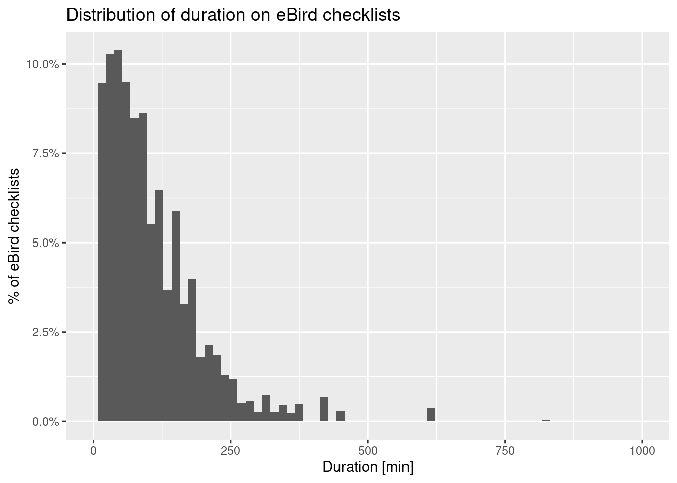
Obviously, these are small dataframes and we can just use dplyr directly on R dataframes. However, our use case may involve much larger dataframes that cannot be held in memory. See this section of the eBird Best Practices guide for a discussion of zero-filling. It’s not really relevant for this post other than to point out that zero-filling leads to even bigger data tables.
What about larger datasets?
Depending on how much RAM you have and what kinds of questions you are exploring, it’s not too difficult to find yourself running out of memory when using read_ebd(). Often this manifests itself in an inglorious crashing of R Studio. You might be able to decompose your analysis into smaller chunks based on smaller dataframes and then put the pieces together. But, sometimes, it’s just really nice to be able to run queries against big datasets, especially when looking at trends over time. Thankfully, there are options.
dbplyr and DBI
The dbplyr package has been around for a long time and allows you to use dplyr with a database back end. You can treat remote tables as if they were local to R and write dplyr statements that are converted to SQL and sent off to the database for processing. Calls to dplyr are lazy in the sense that nothing really happens beyond SQL generation until you request bringing results back into R from the database. Interestingly, you don’t even have to do a library(dbplyr) (though, you must install it) as dplyr will use dbplyr automatically when it recognizes you are communicating with a database. This getting started vignette will get you going. The dbplyr package relies on the DBI (Database Interface) package and on specific DBI backends for the database you are using. The vignette has all the details. Whenever dbplyr is loaded, DBI gets loaded.
My original plan was to use dbplyr with a SQLite database as I wanted a simple, no-server, database. While SQLite is terrific, especially as an embedded database for transaction oriented applications, there’s another database that is even better suited for analytical applications such as ours.
DuckDB
DuckDB is a newish analysis focused database engine. It:
- is relational,
- supports SQL,
- does not require a server,
- runs embedded in a host process,
- has no external dependencies,
- is portable,
- is fast,
- designed for analytical query workloads.
They have really committed to working closely with R by creating a drop in replacement for dplyr called duckplyr (see their blog post).
It positions itself as a replacement for things like dbplyr and using SQLite from R but is compatible with dbplyr. It uses the DBI API, which should make it easy to try out and adopt.
The main duckdb package takes a long time to install.
#install.packages("duckdb")Then install duckplyr.
#install.packages("duckplyr")Start out by loading the duckdb library.
library(duckdb)Loading required package: DBIThe DBI package is loaded automatically when duckdb is loaded.
Create an empty, writable, database.
con <- dbConnect(duckdb(), dbdir = "data/ebdsmp_2024519.duckdb", read_only = FALSE)Now, we want to get the observation and sampling event data into the database. Since these are small dataframes, we could simply write them into the database via DBI functions.
dbWriteTable(con, "observations", observations_df, overwrite = TRUE)
dbWriteTable(con, "sampling_events", sampling_events_df, overwrite = TRUE)
Let’s disconnect. Before disconnecting, notice there’s a .wal file with same base name as the .duckdb file. It’s gone after disconnecting.
dbDisconnect(con)
rm(con)
Querying the DuckDB database
Let’s reconnect to the database and then try to do some basic R things with the tables.
con <- dbConnect(duckdb(), dbdir = "data/ebdsmp_2024519.duckdb", read_only = FALSE)Since DuckDB plays nice with dbplyr, we can use the tbl() function to get a dataframe-like object to use with dplyr.
observations <- tbl(con, 'observations')
sampling_events <- tbl(con, 'sampling_events')
Here is a simple select query.
observations %>%
  select(checklist_id, common_name, observation_count) %>%
  head(10)
# Source: SQL [10 x 3]
# Database: DuckDB v0.10.2 [mark@Linux 6.5.0-41-generic:R 4.4.1//home/mark/Documents/projects/merlin/data/ebdsmp_2024519.duckdb]
checklist_id common_name observation_count
<chr> <chr> <int>
1 G12405482 Barred Owl 3
2 G12405614 Red-winged Blackbird 1
3 G12405614 Canada Goose 13
4 G12405614 American Crow 1
5 G12405614 Ring-billed Gull 9
6 G12405614 Black-capped Chickadee 1
7 G12405614 Purple Martin 5
8 G12405614 Common Grackle 9
9 G12405614 Yellow Warbler 1
10 G12405614 European Starling 1The behavior of dplyr can vary depending on what R commands you are doing. In this query, we are using the local dataframe.
observations_df %>%
  select(observation_count) %>%
  summary()
observation_count
Min. : 1.000
1st Qu.: 1.000
Median : 2.000
Mean : 4.295
3rd Qu.: 3.000
Max. :2909.000
NA's :820 In this one, we are using the remote database table.
observations %>%
  select(observation_count) %>%
  summary()
Length Class Mode
src 2 src_duckdb_connection list
lazy_query 12 lazy_select_query listWe need to use collect() to actually force the query to run and bring back results.
observations %>%
  select(observation_count) %>%
  collect() %>%
  summary()
observation_count
Min. : 1.000
1st Qu.: 1.000
Median : 2.000
Mean : 4.295
3rd Qu.: 3.000
Max. :2909.000
NA's :820 We can list the fields in a table like this.
dbListFields(con, 'observations') [1] "checklist_id" "global_unique_identifier"
[3] "last_edited_date" "taxonomic_order"
[5] "category" "taxon_concept_id"
[7] "common_name" "scientific_name"
[9] "exotic_code" "observation_count"
[11] "breeding_code" "breeding_category"
[13] "behavior_code" "age_sex"
[15] "country" "country_code"
[17] "state" "state_code"
[19] "county" "county_code"
[21] "iba_code" "bcr_code"
[23] "usfws_code" "atlas_block"
[25] "locality" "locality_id"
[27] "locality_type" "latitude"
[29] "longitude" "observation_date"
[31] "time_observations_started" "observer_id"
[33] "sampling_event_identifier" "protocol_type"
[35] "protocol_code" "project_code"
[37] "duration_minutes" "effort_distance_km"
[39] "effort_area_ha" "number_observers"
[41] "all_species_reported" "group_identifier"
[43] "has_media" "approved"
[45] "reviewed" "reason"
[47] "trip_comments" "species_comments" All right, let’s do a simple aggregate query and see which bird is most commonly listed.
observations %>%
  group_by(common_name) %>%
  summarize(
    n = n()
  ) %>%
  arrange(desc(n))
# Source: SQL [?? x 2]
# Database: DuckDB v0.10.2 [mark@Linux 6.5.0-41-generic:R 4.4.1//home/mark/Documents/projects/merlin/data/ebdsmp_2024519.duckdb]
# Ordered by: desc(n)
common_name n
<chr> <dbl>
1 American Robin 1010
2 Red-winged Blackbird 869
3 Blue Jay 749
4 Song Sparrow 724
5 Mourning Dove 678
6 Northern Cardinal 666
7 Common Grackle 617
8 Canada Goose 598
9 Yellow Warbler 598
10 Red-eyed Vireo 588
# ℹ more rowsIf you want to use the duckplyr engine instead of dplyr, just load the library. You’ll get a message about duckplyr methods overwriting the standard dplyr methods and what you can do to restore the dplyr versions.
library(duckplyr)✔ Overwriting dplyr methods with duckplyr methods.
ℹ Turn off with `duckplyr::methods_restore()`.
Attaching package: 'duckplyr'The following objects are masked from 'package:stats':
filter, lagThe following objects are masked from 'package:base':
intersect, setdiff, setequal, unionobservations %>%
group_by(common_name) %>%
summarize(
n = n()
) %>%
arrange(desc(n))# Source: SQL [?? x 2]
# Database: DuckDB v0.10.2 [mark@Linux 6.5.0-41-generic:R 4.4.1//home/mark/Documents/projects/merlin/data/ebdsmp_2024519.duckdb]
# Ordered by: desc(n)
common_name n
<chr> <dbl>
1 American Robin 1010
2 Red-winged Blackbird 869
3 Blue Jay 749
4 Song Sparrow 724
5 Mourning Dove 678
6 Northern Cardinal 666
7 Common Grackle 617
8 Canada Goose 598
9 Yellow Warbler 598
10 Red-eyed Vireo 588
# ℹ more rowsHard to tell if there’s a performance difference since we only have ~30K records. Later we’ll do this with larger data tables.
To “turn off” duckplyr:
duckplyr::methods_restore()ℹ Restoring dplyr methods.Ok, so dplyr is fully capable of interacting with DuckDB database tables via dbplyr and its tbl() function. But, to use DuckDB’s query engine, we load duckplyr to replace dplyr and it creates the query recipe for DuckDB databases. Even without loading the duckplyr library, we can use its DuckDB engine by passing a regular dataframe to duckplyr::as_duckplyr_df().
dbDisconnect(con)
rm(observations, sampling_events, ebdsmp, con)
Time to try loading a whole lot of eBird data into a DuckDB database.
Reading large eBird CSV files into DuckDB using R
If we have giant CSV files, we don’t want to have to load them into an R dataframe and then use DBI to write them to the DuckDB database - the whole reason we might be using DuckDB is because the data won’t fit into memory.
So, let’s assume we have already done an auk_filter which has generated the observations and sampling events text files. These files are:
- tab delimited,
- include all of the columns,
- have capitalized column names with some including spaces.
We can’t bypass R and directly read these into DuckDB using SQL (optionally with DuckDB’s read_csv function) for several reasons. If we need zero-filled observation data we we need to run auk_zerofill. However, the output of this will be an auk_zerofill object containing the two modified dataframes (or a single dataframe if collapse = TRUE is used). These dataframes will likely be too large for R to handle.
Similarly, it’s the read_ebd() and read_sampling() steps (both are auk functions) that do the:
- column name and data type cleanup
- shared checklist collapsing
- taxonomic rollup
We do NOT want to store the raw (or filtered raw) data in a DuckDB database since we want to query data that has been properly had the checklists collapsed and the taxonomic rollup done.
I guess we could bypass R if we rewrote the logic in SQL for zero filling, shared checklist collapsing, taxonomic rollup and column name and datatype changes. That doesn’t sound super fun to do or maintain but is certainly doable.
So, it seems like a viable approach is to break up the eBird downloaded text files into a series of smaller text files and use DBI to append the data to the appropriate tables in the DuckDB database. This will work but there are some challenges.
Creating and populating a DuckDB database
After downloading data from eBird, we have two text files. The first file contains the observation data (one record per species per checklist) and is about 12.3Gb. It includes all checklist observations from the state of Michigan. The second file contains the sampling event data (one record per checklist) and is about 650Mb. We are not going to be able to do a read_ebd() on a 12Gb file (at least I’m not able to on my laptop).
# Set the filenames for the checklist and sample data
f_ebd <- 'data/ebd_US-MI_smp_relMay-2024/ebd_US-MI_smp_relMay-2024.txt'
f_smp <- 'data/ebd_US-MI_smp_relMay-2024/ebd_US-MI_smp_relMay-2024_sampling.txt'

# Create ebd object
ebdsmp <- auk_ebd(f_ebd, file_sampling = f_smp)
Our basic strategy is to grab one month of data at a time using auk and output it as separate monthly text files. As part of our auk filtering we will only include complete checklists. Other than that, the resulting text files have the same format as the EDB downloaded data. We are using the EBD dataset that was released in June of 2024 and contains data up through May, 2024. The files are being written to the data/ebd_US-MI_chunked/ directory.
rerun <- FALSE # Set to TRUE to rerun this code
start_year <- 2015
end_year <- 2024
end_month <- 5

if (rerun) {
  list_years <- seq(start_year, end_year)

  for (list_year in list_years) {
    for (list_month in seq(1, 12)){
      if (list_year <= end_year - 1 | list_month <= end_month) {
        # Create data range to use in auk filter
        start_date <- make_date(year=list_year, month=list_month, day=1L)
        end_date <- ceiling_date(start_date, unit="month") - 1
        print(c(start_date, end_date))

        # Create output filenames based on month and year
        file_ebd <- file.path('data/ebd_US-MI_chunked', paste0('ebd_filtered_MI_', list_year, list_month, '.txt'))
        file_sampling <- file.path('data/ebd_US-MI_chunked', paste0('sampling_filtered_MI_', list_year, list_month, '.txt'))

        # Do the auk filtering
        ebdsmp %>%
          # country: codes and names can be mixed; case insensitive
          auk_state(state = c("US-MI")) %>%
          # date: use standard ISO date format `"YYYY-MM-DD"` with * for wildcard
          auk_date(date = c(start_date, end_date)) %>%
          # complete: all species seen or heard are recorded (this field is in ebd)
          auk_complete() %>%
          # This final step triggers the actual file processing output writing
          auk_filter(file = file_ebd, file_sampling = file_sampling, overwrite = TRUE)
      }
    }
  }
}
Now we want to load each monthly text file into a DuckDB database. The observation files will get appended to an observations table and the sampling event files to a sampling_events table. As of now, these tables don’t exist - actually the entire database doesn’t exist. An easy way to create the tables is to just use dbWriteTable() to load small dataframes to a newly created empty database. In this way, the dataframe acts as a template for the column names and data types. This works as long as you use a data sample file that does not trigger any import parsing related warnings when read with read_ebd() or read_sampling(). So, we’ll use the existing observations_df and sampling_events_df dataframes that we created earlier based on the 2024-05-19 checklist data.
rerun <- FALSE # WARNING: If you rerun this chunk, you will delete any data already in the database

con <- dbConnect(duckdb(), dbdir = "data/ebdsmp_MI_relMay2024.duckdb", read_only = FALSE)

if (rerun) {

  # Filenames of text files to use as table templates
  file_ebd <- "data/ebd_20240519_MI.txt"
  file_sampling <- "data/smp_20240519_MI.txt"

  sampling_events_df <- read_sampling(file_sampling, unique = TRUE)
  DBI::dbCreateTable(con, 'sampling_events', sampling_events_df)
  # Remove the local sampling events dataframe
  rm(sampling_events_df)

  observations_df <- read_ebd(file_ebd, unique = TRUE)
  # Change observation_count to integer
  observations_df$observation_count <- as.integer(observations_df$observation_count)
  DBI::dbCreateTable(con, 'observations', observations_df)
  # Remove the local observations dataframe
  rm(observations_df)

  # Delete all records from the two tables
  dbExecute(con, "DELETE FROM observations")
  dbExecute(con, "DELETE FROM sampling_events")
}
At this point we have a new DuckDB database with two empty tables that are ready to receive data. Use DBI::dbColumnInfo() to see table structures. Make sure you include the LIMIT clause if you attempt to do this after loading all of your data. Otherwise, you are inviting an R Studio crash.
rs <- dbSendQuery(con, "SELECT * FROM sampling_events LIMIT 10")
DBI::dbColumnInfo(rs)
name type
1 checklist_id character
2 last_edited_date character
3 country character
4 country_code character
5 state character
6 state_code character
7 county character
8 county_code character
9 iba_code character
10 bcr_code integer
11 usfws_code character
12 atlas_block character
13 locality character
14 locality_id character
15 locality_type character
16 latitude numeric
17 longitude numeric
18 observation_date Date
19 time_observations_started character
20 observer_id character
21 sampling_event_identifier character
22 protocol_type character
23 protocol_code character
24 project_code character
25 duration_minutes integer
26 effort_distance_km numeric
27 effort_area_ha numeric
28 number_observers integer
29 all_species_reported logical
30 group_identifier character
31 trip_comments characterAlright, let’s load all of our data! This next step is quite time consuming.
rerun <- FALSE # Set to TRUE to rerun this code
start_year <- 2015
end_year <- 2024
end_month <- 5

if (rerun) {
  # Make sure tables are empty before we begin
  dbExecute(con, "DELETE FROM observations")
  dbExecute(con, "DELETE FROM sampling_events")

  list_years <- seq(start_year, end_year)
  list_months <- seq(1, 12)

  for (list_year in list_years) {
    for (list_month in list_months) {

      # Create filenames of source text files
      file_ebd <- file.path('data/ebd_US-MI_chunked', paste0('ebd_filtered_MI_', list_year, list_month, '.txt'))
      file_sampling <- file.path('data/ebd_US-MI_chunked', paste0('sampling_filtered_MI_', list_year, list_month, '.txt'))

      if (list_year <= end_year - 1 | list_month <= end_month) {
        start_date <- make_date(year=list_year, month=list_month, day=1L)
        end_date <- ceiling_date(start_date, unit="month") - 1
        print(c(start_date, end_date))

        # Create and append dataframe to the sampling_events table
        sampling_events_df <- read_sampling(file_sampling, unique = TRUE)
        dbAppendTable(con, "sampling_events", sampling_events_df)
        rm(sampling_events_df)

        # Create and append dataframe to the observations table
        observations_df <- read_ebd(file_ebd, unique = TRUE)
        # Change observation_count to integer
        observations_df$observation_count <- as.integer(observations_df$observation_count)

        dbAppendTable(con, "observations", observations_df)
        rm(observations_df)
    }
  }
  }


}
The populated database is ~1.3Gb.
Analyzing eBird data in the DuckDB database
Let’s see how many total records we have.
dbGetQuery(con, "SELECT COUNT(*) FROM sampling_events") count_star()
1 1529700dbGetQuery(con, "SELECT COUNT(*) FROM observations") count_star()
1 21664757A subtle problem with duplicate checklist_id’s
Through using auk::read_ebd() and auk::read_sampling(), important preprocessing was done such as collapsing shared checklists and rolling up observations to the species level. One might think that we wouldn’t have to worry about duplicate checklist_id values. Well, we do.
dbGetQuery(con, "SELECT checklist_id
           FROM sampling_events
           GROUP BY checklist_id
           HAVING COUNT(checklist_id) > 1")
checklist_id
1 G1475849
2 G7107571
3 G10713331
4 G4962093
5 G5729899
6 G2040552
7 G4385780
8 G8521612
9 G10019302
10 G7107956
11 G7107583Turns out we have eleven duplicate checklist_id values and they are all shared checklists. What? I was surprised as well when I found this, but it wasn’t too hard to figure out what’s going on. Let’s look at one the duplicate checklists.
dbGetQuery(con,"SELECT checklist_id, observation_date, locality_id, sampling_event_identifier, observer_ID FROM sampling_events WHERE checklist_id = 'G7107571';") checklist_id observation_date locality_id sampling_event_identifier
1 G7107571 2021-06-27 L2123031 S93447285
2 G7107571 2021-07-05 L2123031 S93447235
observer_id
1 obsr123074
2 obsr351872A few things to note:
- the
observation_datevalues are different, AND they span a month boundary, - the
observer_idvalues are different, - neither
sampling_event_identifiercontains the comma concatenated list of identifiers.
We might infer that these two individuals were birding together and one of them entered an incorrect date into eBird. That actually seems like it could be a pretty common occurrence, yet we only got eleven such duplicates out of millions of records for Michigan. The issue is caused by our “chunking” of the giant download file into monthly pieces so as to be able to load it via R into the DuckDB database. Had we chunked the data by year, instead of by month and year, this duplicate checklist_id would not have occurred. The auk::read_sampling() function would have collapsed them into a single records using some sort of logic to decide which record to keep. Of course, even chunking by year doesn’t guarantee no duplicate checklist_id values.
dbGetQuery(con,"SELECT checklist_id, group_identifier, observation_date, sampling_event_identifier, observer_ID, last_edited_date FROM sampling_events WHERE checklist_id = 'G1475849';") checklist_id group_identifier observation_date sampling_event_identifier
1 G1475849 G1475849 2015-11-20 S25919906,S25968002
2 G1475849 G1475849 2016-02-25 S27899045
observer_id last_edited_date
1 obsr653314,obsr428042 2021-03-26 03:17:06.584504
2 obsr653323 2021-03-26 03:17:06.584504Again, I’m guessing we had a group of three birders, one of whom put in the wrong date (by a lot), yet somehow the last_edited_date values are identical (and several years later). Maybe.
I guess we need to dig into the actual R code in auk to see how such cases are handled. The source file we need to explore is auk-unique.r. It appears that the “tiebreaker” is whichever record has the lowest sampling_event_identifier value. Regardless, we are in a bit of pickle as we can’t simply use read_sampling() and read_ebd() on our 12Gb file. But, if we chunk the data, we can’t ensure no duplicate checklist_id values. Furthermore, these are just the records we caught due to our chunking. No idea how many such duplicate records with inconsistent observation dates there are.
We will just do something consistent with the current auk_unique() function and keep the record with the lowest sampling_event_identifier value.
dup_checklist_ids <- dbGetQuery(con, "SELECT checklist_id, min(sampling_event_identifier) as sei
           FROM sampling_events
           GROUP BY checklist_id
           HAVING COUNT(checklist_id) > 1")

dup_checklist_ids
checklist_id sei
1 G4962093 S64297187
2 G5729899 S73905868,S73907623
3 G4385780 S58370794
4 G7107583 S93447555,S93459182
5 G2040552 S32581769
6 G8521612 S112297874
7 G7107571 S93447235
8 G1475849 S25919906,S25968002
9 G10713331 S147457082
10 G7107956 S93453425,S93459174
11 G10019302 S134105819Now we want to delete rows that match the each checklist_id but do not match the sampling_event_identifier.
for(i in 1:nrow(dup_checklist_ids)) {
    checklist_id <- dup_checklist_ids[i,1]
    sei <- dup_checklist_ids[i,2]

    sql_del_sampling <- paste0("DELETE FROM sampling_events WHERE checklist_id == '", checklist_id, "' and sampling_event_identifier != '", sei, "';")

    sql_del_obs <- paste0("DELETE FROM observations WHERE checklist_id == '", checklist_id, "' and sampling_event_identifier != '", sei, "';")

    print(sql_del_sampling)
    dbExecute(con, sql_del_sampling)
    print(sql_del_obs)
    dbExecute(con, sql_del_obs)
}
[1] "DELETE FROM sampling_events WHERE checklist_id == 'G4962093' and sampling_event_identifier != 'S64297187';"
[1] "DELETE FROM observations WHERE checklist_id == 'G4962093' and sampling_event_identifier != 'S64297187';"
[1] "DELETE FROM sampling_events WHERE checklist_id == 'G5729899' and sampling_event_identifier != 'S73905868,S73907623';"
[1] "DELETE FROM observations WHERE checklist_id == 'G5729899' and sampling_event_identifier != 'S73905868,S73907623';"
[1] "DELETE FROM sampling_events WHERE checklist_id == 'G4385780' and sampling_event_identifier != 'S58370794';"
[1] "DELETE FROM observations WHERE checklist_id == 'G4385780' and sampling_event_identifier != 'S58370794';"
[1] "DELETE FROM sampling_events WHERE checklist_id == 'G7107583' and sampling_event_identifier != 'S93447555,S93459182';"
[1] "DELETE FROM observations WHERE checklist_id == 'G7107583' and sampling_event_identifier != 'S93447555,S93459182';"
[1] "DELETE FROM sampling_events WHERE checklist_id == 'G2040552' and sampling_event_identifier != 'S32581769';"
[1] "DELETE FROM observations WHERE checklist_id == 'G2040552' and sampling_event_identifier != 'S32581769';"
[1] "DELETE FROM sampling_events WHERE checklist_id == 'G8521612' and sampling_event_identifier != 'S112297874';"
[1] "DELETE FROM observations WHERE checklist_id == 'G8521612' and sampling_event_identifier != 'S112297874';"
[1] "DELETE FROM sampling_events WHERE checklist_id == 'G7107571' and sampling_event_identifier != 'S93447235';"
[1] "DELETE FROM observations WHERE checklist_id == 'G7107571' and sampling_event_identifier != 'S93447235';"
[1] "DELETE FROM sampling_events WHERE checklist_id == 'G1475849' and sampling_event_identifier != 'S25919906,S25968002';"
[1] "DELETE FROM observations WHERE checklist_id == 'G1475849' and sampling_event_identifier != 'S25919906,S25968002';"
[1] "DELETE FROM sampling_events WHERE checklist_id == 'G10713331' and sampling_event_identifier != 'S147457082';"
[1] "DELETE FROM observations WHERE checklist_id == 'G10713331' and sampling_event_identifier != 'S147457082';"
[1] "DELETE FROM sampling_events WHERE checklist_id == 'G7107956' and sampling_event_identifier != 'S93453425,S93459174';"
[1] "DELETE FROM observations WHERE checklist_id == 'G7107956' and sampling_event_identifier != 'S93453425,S93459174';"
[1] "DELETE FROM sampling_events WHERE checklist_id == 'G10019302' and sampling_event_identifier != 'S134105819';"
[1] "DELETE FROM observations WHERE checklist_id == 'G10019302' and sampling_event_identifier != 'S134105819';"dbGetQuery(con, "SELECT COUNT(*) FROM sampling_events") count_star()
1 1529700Yep, this is 11 records less than we had before. This next query should return no rows.
dbGetQuery(con, "SELECT checklist_id
           FROM sampling_events
           GROUP BY checklist_id
           HAVING COUNT(checklist_id) > 1")
[1] checklist_id
<0 rows> (or 0-length row.names)Using dbplyr and dplyr
Now let’s do some querying. We’ll start by using dplyr.
observations <- tbl(con, 'observations')
sampling_events <- tbl(con, 'sampling_events')
Printing observations should just result in a few rows returned.
observations# Source: table<observations> [?? x 48]
# Database: DuckDB v0.10.2 [mark@Linux 6.5.0-41-generic:R 4.4.1//home/mark/Documents/projects/merlin/data/ebdsmp_MI_relMay2024.duckdb]
checklist_id global_unique_identi…¹ last_edited_date taxonomic_order category
<chr> <chr> <chr> <dbl> <chr>
1 G1088065 URN:CornellLabOfOrnit… 2024-01-11 12:1… 324 species
2 G1088065 URN:CornellLabOfOrnit… 2024-01-11 12:1… 8312 species
3 G1088065 URN:CornellLabOfOrnit… 2024-01-11 12:1… 33967 species
4 G1088065 URN:CornellLabOfOrnit… 2024-01-11 12:1… 21168 species
5 G1088065 URN:CornellLabOfOrnit… 2024-01-11 12:1… 11175 species
6 G1088065 URN:CornellLabOfOrnit… 2024-01-11 12:1… 11527 species
7 G1088065 URN:CornellLabOfOrnit… 2024-01-11 12:1… 31790 species
8 G1088065 URN:CornellLabOfOrnit… 2024-01-11 12:1… 32595 species
9 G1088065 URN:CornellLabOfOrnit… 2024-01-11 12:1… 6479 species
10 G1088065 URN:CornellLabOfOrnit… 2024-01-11 12:1… 10979 species
# ℹ more rows
# ℹ abbreviated name: ¹global_unique_identifier
# ℹ 43 more variables: taxon_concept_id <chr>, common_name <chr>,
# scientific_name <chr>, exotic_code <chr>, observation_count <int>,
# breeding_code <chr>, breeding_category <chr>, behavior_code <chr>,
# age_sex <chr>, country <chr>, country_code <chr>, state <chr>,
# state_code <chr>, county <chr>, county_code <chr>, iba_code <chr>, …Let’s redo our common species query.
common_species <- observations %>%
  group_by(common_name) %>%
  summarize(
    n = n()
  ) %>%
  arrange(desc(n))
We can see the SQL generated by dbplyr:
common_species %>% show_query()<SQL>
SELECT common_name, COUNT(*) AS n
FROM observations
GROUP BY common_name
ORDER BY n DESCUse collect() to actually run the query and bring back results.
common_species %>% dplyr::collect() # Making sure not using duckplyr::collect()# A tibble: 431 × 2
common_name n
<chr> <dbl>
1 Blue Jay 723625
2 Black-capped Chickadee 714290
3 American Robin 701454
4 Northern Cardinal 673327
5 Mourning Dove 607148
6 American Crow 587172
7 American Goldfinch 568616
8 Red-winged Blackbird 560814
9 Canada Goose 543752
10 Downy Woodpecker 527761
# ℹ 421 more rowsWhat about common date functions? There are multiple ways to work with dates and times:
- many
lubridatefunctions are supported bydbplyrandduckplyr, - we can use the
sql()function to wrap SQL bits to pass to DuckDB (which supports a bunch of datetime functions.)
For example, here’s what dbplyr does with the lubridate::year() function.
dbplyr::translate_sql(year(observation_date), con = con)<SQL> EXTRACT(year FROM observation_date)Let’s extend our common species query to group by year. A good approach seems to be to use mutate to compute the column you want to group on. Not only does this provide an easy way to name the computed column but I’ve also had trouble using lubridate functions directly in group by statements.
common_species_yearly <- observations %>%
  mutate(ebdyear = year(observation_date)) %>%
  group_by(ebdyear, common_name) %>%
  summarize(
    n = n()
  ) %>%
  arrange(ebdyear, desc(n))

common_species_yearly %>% show_query()
`summarise()` has grouped output by "ebdyear". You can override using the
`.groups` argument.<SQL>
SELECT ebdyear, common_name, COUNT(*) AS n
FROM (
SELECT observations.*, EXTRACT(year FROM observation_date) AS ebdyear
FROM observations
) q01
GROUP BY ebdyear, common_name
ORDER BY ebdyear, n DESCcommon_species_yearly %>% dplyr::collect()`summarise()` has grouped output by "ebdyear". You can override using the
`.groups` argument.# A tibble: 3,512 × 3
# Groups: ebdyear [10]
ebdyear common_name n
<dbl> <chr> <dbl>
1 2015 Black-capped Chickadee 34584
2 2015 Blue Jay 33924
3 2015 American Robin 32854
4 2015 American Crow 31872
5 2015 Northern Cardinal 30726
6 2015 American Goldfinch 28319
7 2015 Mourning Dove 27910
8 2015 Canada Goose 27614
9 2015 Mallard 27196
10 2015 Red-winged Blackbird 26268
# ℹ 3,502 more rowsLet’s try a similar approach but use DuckDB’s datepart function.
common_species_yearly <- observations %>%
  mutate(ebdyear = sql("datepart('year', observation_date)")) %>%
  group_by(ebdyear, common_name) %>%
  summarize(
    n = n()
  ) %>%
  arrange(ebdyear, desc(n))

common_species_yearly %>% show_query()
`summarise()` has grouped output by "ebdyear". You can override using the
`.groups` argument.<SQL>
SELECT ebdyear, common_name, COUNT(*) AS n
FROM (
SELECT observations.*, datepart('year', observation_date) AS ebdyear
FROM observations
) q01
GROUP BY ebdyear, common_name
ORDER BY ebdyear, n DESCcommon_species_yearly %>% collect()`summarise()` has grouped output by "ebdyear". You can override using the
`.groups` argument.# A tibble: 3,512 × 3
# Groups: ebdyear [10]
ebdyear common_name n
<dbl> <chr> <dbl>
1 2015 Black-capped Chickadee 34584
2 2015 Blue Jay 33924
3 2015 American Robin 32854
4 2015 American Crow 31872
5 2015 Northern Cardinal 30726
6 2015 American Goldfinch 28319
7 2015 Mourning Dove 27910
8 2015 Canada Goose 27614
9 2015 Mallard 27196
10 2015 Red-winged Blackbird 26268
# ℹ 3,502 more rowsDoes duckplyr support lubridate directly?
library(duckplyr)common_species_yearly_duckplyr <- observations %>%
mutate(ebdyear = year(observation_date)) %>%
group_by(ebdyear, common_name) %>%
summarize(
n = n()
) %>%
arrange(ebdyear, desc(n))
common_species_yearly_duckplyr %>% show_query()`summarise()` has grouped output by "ebdyear". You can override using the
`.groups` argument.<SQL>
SELECT ebdyear, common_name, COUNT(*) AS n
FROM (
SELECT observations.*, EXTRACT(year FROM observation_date) AS ebdyear
FROM observations
) q01
GROUP BY ebdyear, common_name
ORDER BY ebdyear, n DESCcommon_species_yearly_duckplyr %>% collect()`summarise()` has grouped output by "ebdyear". You can override using the
`.groups` argument.# A tibble: 3,512 × 3
# Groups: ebdyear [10]
ebdyear common_name n
<dbl> <chr> <dbl>
1 2015 Black-capped Chickadee 34584
2 2015 Blue Jay 33924
3 2015 American Robin 32854
4 2015 American Crow 31872
5 2015 Northern Cardinal 30726
6 2015 American Goldfinch 28319
7 2015 Mourning Dove 27910
8 2015 Canada Goose 27614
9 2015 Mallard 27196
10 2015 Red-winged Blackbird 26268
# ℹ 3,502 more rowsYes, it does!
Let’s finish with a summary of birding effort by year for the month of May in Iosco County.
sampling_events %>%
  mutate(ebdyear = year(observation_date), ebdmonth = month(observation_date)) %>%
  filter(ebdmonth == 5, county == 'Iosco') %>%
  group_by(ebdyear) %>%
  summarize(
    mean_distance = mean(effort_distance_km),
    mean_duration = mean(duration_minutes),
    num_checklists = n()
  ) %>%
  collect()
Warning: Missing values are always removed in SQL aggregation functions.
Use `na.rm = TRUE` to silence this warning
This warning is displayed once every 8 hours.# A tibble: 10 × 4
ebdyear mean_distance mean_duration num_checklists
<dbl> <dbl> <dbl> <dbl>
1 2015 3.60 135. 672
2 2016 3.36 130. 952
3 2017 2.93 133. 969
4 2018 3.65 127. 1201
5 2019 3.46 131. 1365
6 2020 4.01 125. 701
7 2021 3.52 125. 1673
8 2022 3.23 123. 1667
9 2023 3.28 121. 1772
10 2024 3.42 122. 1960Now that we’ve got our Michigan data in a DuckDB database, it should be easier to do more analysis. Future blogs posts are planned on this topic.
Some DuckDB Resources
Here are a few resources for learning more about DuckDB and duckplyr.
Citation
BibTeX citation:
@online{isken2024,
  author = {Isken, Mark},
  title = {Create an {eBird} {DuckDB} Database for Use with {R}},
  date = {2024-06-24},
  url = {https://bitsofanalytics.org/posts/ebird_duckdb/duckdb_create_database.html},
  langid = {en}
}
For attribution, please cite this work as:
Isken, Mark. 2024. “Create an eBird DuckDB Database for Use with
R.” June 24. https://bitsofanalytics.org/posts/ebird_duckdb/duckdb_create_database.html.